1. Introduction

There has been growing interests in engineering dynamics in modelling systems that are chaotic. Chaos is an aspect of nonlinear dynamics that is concerned with systems governed by equations in which a small change in one variable can induce a large systematic change. The relevance of the understanding of chaos in nonlinear electrical circuits, Duffing oscillating systems, magneto-mechanical devices, weather and climate, fluid flow in some systems and host of others cannot be overstressed. Therefore, it is germane to emphasize the adoption of visual tools such as chaos diagrams to enrich understanding of chaotic behaviour. Useful tools for detecting chaos have been explained by[2]. To observe the state variables (time series), the phase portrait, the Poincare map, the power spectrum, the Lyapunov exponents and bifurcation diagram are used to detect chaos in dynamical systems. In the paper, the authors adopted all these tools using chaotic driven pendulum as a case study. The paper clearly explains the existence of chaos in driven pendulum using all methods mentioned. The Simulation results obtained from all the tools concur with each other. Also, control of chaos in driven pendulum was realized in the study. Thepaper sufficiently demonstrates the usefulness of bifurcation diagram which is one of the most important chaos diagrams for explaining chaos. Chaos researchers have identified that DC–DC converter is a highly nonlinear system. It is observed that DC–DC converters are experiencing bifurcation and chaotic oscillations. In their paper,[3] studied and analysed chaos as well as bifurcation of voltage mode controlled DC–DC buck converter. The study revealed that such DC–DC buck converter is experiencing a chaotic behaviour under certain operation conditions. The paper studied the bifurcation and chaos in the DC–DC buck converter by changing different control parameters. The authors demonstrated satisfactorily how bifurcation diagrams and state–space diagrams can be shown for these parameters. It is well known that horizontal platform system (HPS) is usually applied in offshore and earthquake technology but unfortunately, it is difficult and time-consuming for regulation. In order to understand the nonlinear dynamic behaviour of HPS and reduce the cost when using it,[4] employs differential transformation method to study the bifurcation behaviour of HPS. Their numerical results showed a complex dynamic behaviour comprising periodic, sub-harmonic, and chaotic responses. Furthermore, their results reveal the changes which take place in the dynamic behaviour of the HPS as the external torque is increased. The paper concluded that the proposed method provides an effective means of gaining insights into the nonlinear dynamics of horizontal platform system.[5] Investigated the periodic motions of a non-linear geared rotor-bearing system using the incremental harmonic balance (IHB) method. A path following procedure using arc length continuation technique was used to trace the bifurcation diagrams. The system exhibited a period doubling route and a quasiperiodic route to chaos in different regions of excitation frequency. The chaotic motions are investigated by numerical integration and the Lyapunov exponents are computed. The paper concluded that the periodic solutions and sub-harmonic solutions obtained by the IHB method compares very well with those obtained by numerical integration. Bifurcation and chaos in a 4-side simply supported rectangular thin electro-magneto-elastic plate in electro-magnetic, mechanical and temperature fields was studied by[6]. Based on the basic nonlinear electro-magneto-elastic motion equations for a rectangular thin plate and expressions of electromagnetic forces, vibration equations are derived for the mechanical loading in a nonlinear temperature field and a steady transverse magnetic field. By using Melnikov function method, the criteria are obtained for chaos motion to exist as demonstrated by the Smale horseshoe mapping. The vibration equations are solved numerically by using a fourth-order Runge-Kutta method. Its bifurcation diagram, Lyapunov exponents diagram, displacement wave diagram, phase diagram and Poincare section diagram are obtained for some examples. The characteristics of the vibration system were analysed, and the roles of parameters on the systems are clearly understood.

The use of Runge-Kutta methods have provided a reliable alternative numerical tools for producing fractals, phase plots, bifurcation diagrams and other forms of chaos diagrams.[7] Carried out a critical review on the development of Runge-Kutta discontinuous Galerkin (RKDG) methods for nonlinear convection-dominated problems. The authors combined a special class of Runge-Kutta time discretization that allows the method to be nonlinearly stable regardless of its accuracy, with a finite element space discretization by discontinuous approximations that incorporates the idea of numerical fluxes and slope limiters coined during the remarkable development of high-resolution finite difference and finite volume schemes. The findings of this review revealed that RKDG methods are stable, high-order accurate and highly parallelizable schemes that can easily handle complicated geometries and boundary conditions. The review showed its immense applications in Navier-Stokes equations and Hamilton-Jacobian equations. This study has become a breakthrough in computational fluid dynamics especially in producing its chaos diagrams.[8] demonstrated how Duffing’s equation can be applied in predicting the emission characteristics of sawdust particles. The paper explains the modelling of sawdust particle motion as a two dimensional transformation system of continuous time series. The authors applied Runge-Kutta algorithms in providing solution to Duffing’s model equation for the sawdust particles. The author simulation results revealed a high profile feasibility of modelling sawdust dynamics as emissions from band saws. The conclusion drawn from this work was that the findings no doubt provide a breakthrough in the knowledge of sawdust emission technology.[9] article in 2002 investigated the chaotic behaviour of a transformer during ferroresonance under single and double opens conductor configurations .The solutions of the nonlinear differential equations which describe a ferroresonant circuit were categorized into three types, i.e., periodic, quasiperiodic, and chaotic. Simulation of each of these types was carried out using the fourth order Runge-Kutta method and results were corroborated using EMTP. The results revealed that the type of response from both configurations is influenced by the transformer saturation characteristic, core loss, and the amplitude of the voltage source. However, the double open conductor configuration exhibits greater sensitivity to parameters and chaotic behaviour for lower values of voltage source. The paper asserted that the steady state bifurcation diagram generated using a continuation procedure reveals the occurrence of contiguous stable and unstable fundamental frequency solutions. A critical study was carried out by[10] on the systematic analysis of the dynamic behaviour of the hybrid squeeze-film damper (HSFD) mounted on a gear-bearing system with strongly non-linear oil-film force and gear meshing force. The dynamic orbits of the system were observed using bifurcation diagrams plotted using the dimensionless unbalance coefficient, damping coefficient and the dimensionless rotating speed ratio as control parameters. The non-dimensional equations of the gear-bearing system were solved using the fourth order Runge-Kutta method. The onset of chaotic motion was identified from the chaotic diagrams which are phase diagrams, power spectra, Poincaré maps, bifurcation diagrams, maximum Lyapunov exponents and fractal dimension of the gear-bearing system. The research outcome provides some useful insights into the design and development of a gear-bearing system for rotating machinery that operates in highly rotating speed and highly non-linear regimes. Chaotic vibrations of a harmonically excited non-linear oscillator with Coulomb damping were investigated by numerical solution in a range of excitation frequencies[11]. The paper reported that phase plane diagrams, Poincaré maps and time histories were obtained with the Poincaré maps exhibiting strange attractor behaviour. Lyapunov exponents were estimated and for chaos; one of them is positive. A period doubling route to chaos was observed in certain frequency ranges and this was explained by harmonic balance analysis

[12] Emphasized that one of the major ways of investigating the dynamics of a continuous time system by differential equation is the use of Runge-Kutta methods in developing bifurcation diagram.

The challenge of relevant literature that explores chaos diagrams as visual aid in dynamics characterization cannot be over emphasised. Furthermore, extensive literature study has shown significantly that Runge-Kutta is one of the most versatile numerical techniques that are used in computing chaos problems. A careful perusal of the numerous literatures consulted shows that there exists a lacuna. There is still a question of which of the Runge-Kutta orders (i.e First, Second, Third, Fourth, Fifth and Sixth orders) provides acceptable and reliable chaos diagrams. Therefore, the benefits of comparative analysis of fourth-order and fifth- order numerically computed chaos diagrams cannot be overemphasized. This paper intend to fill part of the identified gaps by comparing the reliability of fourth and fifth orders Runge-Kutta methods in producing chaos diagrams for Duffing oscillator using[1] as a reference standard.

2. Methodology

2.1. Duffing Oscillator

The studied normalized governing equation for the dynamic behaviour of a harmonically excited Duffing system is given by equation (1).

(1)

In equation (1),, and represents respectively displacement, velocity and acceleration of the Duffing oscillator about a set datum. The damping coefficient is. Amplitude strength of harmonic excitation, excitation frequency and time are respectively , and .[1,13,14] proposed that combination of = 0.168, = 0.21, and = 1 .0 or = 0.0168, = 0.09 and = 1.0 parameters leads to chaotic behaviour of a harmonically excited Duffing oscillator. This study investigated the evolution of 1000 trajectories that started very close to each other and over five (5) excitation periods using adaptive Runge-Kutta algorithms with a start time step (). The resulting strange attractor[15] at the end of five (5) excitation periods in addition to other selected parameters combination are characterized with fractal disk dimension estimate based on optimum disk count algorithms.

2.2. Parameter Details of Studied Cases

A studied case is defined same as a parameter point in the parameters space. In all cases was studied in the plane of excitation frequencies versus amplitudes at two different damp coefficient levels ( = 0.168 and = 0.0168). Excitation frequency and amplitude range are and respectively. Common parameters to all cases includes initial displacement range (), Zero initial velocity () and random number generating seed value of 9876

2.3. Attractor Characterization

The optimum disk count algorithm was used to characterize all the resulting attractors based on fifteen (15) different disk scales of examination and over five (5) independent trials. The Duffing behaviour is taken to be chaotic for estimated disk dimension greater than one (1.0) and otherwise non-chaotic.

2.4. Time step selection

[16] Argued that employing a constant time step size to seek solutions of ordinary differential equations of some dynamical systems that exhibits an abrupt change could pose serious limitation. In such engineering problems (chaotic dynamics) of interest, the choice of adaptive time step size becomes inevitable. The formula used for increasing and decreasing the time step () in this study is given by (2) and (3) respectively. The tolerance () was fixed at for all computation steps while the error () compares predicted results taking two half-steps with taking a full step. Equation (2) is used when and equation (3) used when.

(2)

(3)

3. Results and Discussions

The algorithms developed by[17] was utilised to generate data for figures 1_(a) to 1_(d) shown below subject to minor modification.

The strange attractors in figure 1 are all qualitatively the same as in the literature; see[1]. Though the estimated fractal disk dimensions (D_E) of the four strange attractors in figure 1 are quantitatively different, the fact that they are greater than one (Chaotic criteria for this study) signifies manifestation of chaotic behaviour of Duffing Oscillator for the respective combined driven parameters. The strange attractors in figure 1_(c) and 1_(d) has higher fractal disk dimension and fill more of the phase space than the attractors in figures 1_(a) and 1_(b). It is expected in line with the definition of dimension as space filling ability of an attractor. 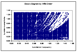Furthermore, major modification of algorithms developed by[17] enable numerical prediction of the Duffing Oscillator behaviour at (10201) case points in the plane of excitation frequencies versus amplitudes. The collection of case points with estimated fractal disk dimension greater than one (1.0) at different damp level forms the chaos diagrams shown in figures 2_(a), 2_(b), 3_(a) and 3_(b).

Figures 2_(a) and 2_(b) are qualitatively alike and likewise figures 3_(a) and 3_(b). Each figure took average of seventeen and half hours to compute on Toshiba laptop Intel (R) Pentium (R) Dual CPU T3400 at 2.16GHz with 2.00GB Ram and 32-bit operating system. There are respectively 6356 (62.3%), 5435 (53.3%), 7943 (77.9%) and 8046 (78.9%) out of 10201 tested parameter points that drives Duffing oscillator chaotically in figures 2_(a) and 2_(b) 3_(a) and 3_(b). In addition ,[18] suggests respectively reliability of chaos diagrams 2(a) and 3(a) than 2(b) and 3(b) because of shorter average computation time step associated with Runge-Kutta fourth order algorithms in comparison with its fifth order counterpart. Probability of chaotic behaviour is non-uniform on the plane ()by visual assessments of figures 2 and 3. However, chaotic behaviour is highly probable below the diagonal line of the excitation frequencies versus amplitudes plane () than above and neighbourhood of the diagonal for all studied cases.

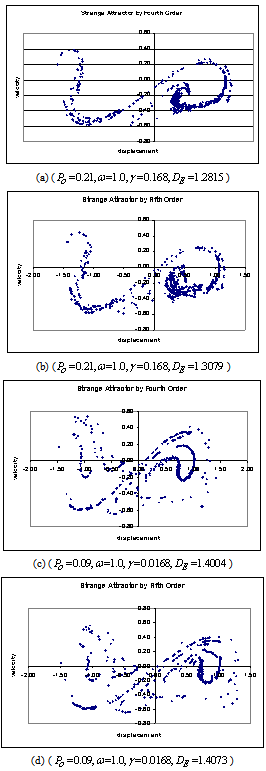Figure 1. Computed strange attractors of Duffing Oscillator at two different damp coefficients based on one thousand trajectories at the end of five excitation periods

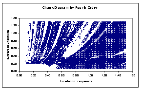Figure 2(a). Chaos diagrams at 0.168 damp coefficients computed by Runge-Kutta fourth order algorithms ()

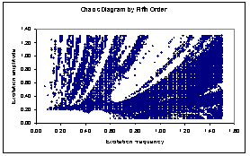Figure 2(b). Chaos diagrams at 0.168 damp coefficients computed by Runge-Kutta fifth order algorithms ()

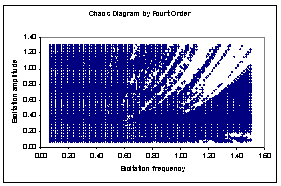Figure 3(a). Chaos diagrams at 0.0168 damp coefficients computed by Runge-Kutta fourth order algorithms ()

Figure 3(b). Chaos diagrams at 0.0168 damp coefficients computed by Runge-Kutta fifth order algorithms ()

4. Conclusions

This study has developed numerical tools that can predict the chaos diagrams of a harmonically excited Duffing Oscillator in the excitation frequencies versus amplitudes using fourth and fifth order Runge-Kutta algorithms. The chaos diagrams compares satisfactorily with literature results. Furthermore, there is qualitative agreement between chaos diagrams generated at different damp coefficients by fourth and fifth order algorithms. The probability that selected excitation frequencies and amplitudes will drive Duffing oscillator chaotically at 0.168 damp coefficient are 62.3% and 53.3% for fourth and fifth order Runge-Kutta algorithms are respectively, 77.9% and 78.9% at 0.0168 damp coefficient. However the utility of these chaos diagrams as tool for searching possible regions of parameter space where chaotic behaviour/motion exist may require additional tests such as spectral analysis, largest positive Lyapunov exponent e.t.c.