Hiroshi Ohsaki 1, Masami Iwase 2, Shoshiro Hatakeyama 2
1Graduate School of Advanced Science and Technology, Tokyo Denki University, Chiyoda-ku, Tokyo, 101-8457, Japan
2Department of Robotics and Mechatronics, Tokyo Denki University, Chiyoda-ku, Tokyo, 101-8457, Japan
Correspondence to: Hiroshi Ohsaki , Graduate School of Advanced Science and Technology, Tokyo Denki University, Chiyoda-ku, Tokyo, 101-8457, Japan.
| Email: |  |
Copyright © 2012 Scientific & Academic Publishing. All Rights Reserved.
Abstract
This study addresses a discretization method with Lebesgue sampling for a type of nonlinear system, and proposes a control method based on the discrete system model. A cart- pendulum system is used as this example. Applying this control method to some real systems, how to implement the controller is a crucial problem. To overcome the problem, an impulsive Luenberger observer is introduced with a numerical forward mapping from the current system state to the one-step ahead state by well-known Runge-Kutta method. As the result, a cart- pendulum system with a quantizer, whose quantization interval is relatively large amount, can be controlled effectively. Numerical simulations are performed to verify the effectiveness of the proposed method.
Keywords:
Lebesgue Sampling Control, Cart-Pendulum, Motion Control
1. Introduction
Discrete-time control has nice properties and is natural for real systems with respect to the implementation viewpoint. This assertion is based on difficulty to realize an arbitrary short sampling interval. That means a control law described in continuous-time systems basically cannot be implemented to real systems as it is, with the exception of analog devices use. Hence, digital control systems with a time-invariant and constant sampling interval are usually utilized to implement a desired control law by some digital devices including computers, DSPs and FPGAs[1].Recently some interesting extensions on the digital control are discussed. Lebesgue sampling is one of such topics. In usual digital control, the update of the control input is performed every sampling interval, and the sampling interval is given by chopping the time axis at some regular intervals. On the other hand, in the Lebesgue sampling case, the update of the control input is performed whenever the output of the system exceeds the given levels which are decided by chopping the output range like chopping the time axis in the usual digital control case[2]. In other words, the control input is updated whenever some events on the output arise. In this sense, the digital control with Lebesgue sampling can be regarded as an event-based control[3,4]. As other related studies, a comparison between periodic and Lebesgue sampling for one-dimensional systems can be found in[5]. In the literature, it is shown that some impusivecontrol based on the Lebesgue sampling may reduce the average sampling frequency to achieve the almost same performance as the periodic sampling case.The concept of the Lebesgue sampling-based control is very natural for systems with many digital sensors such as encoders, and also for networked-systems. Typically we can say cheaper sensors are desired from the cost viewpoint for marketed products such as cars. Such cheaper sensors, however, don't provide good resolution in general, and a typical controller cannot achieve good performance. Hence, there are several studies on observer-based control which considers the quantization effect of low-resolution sensors to recover good control performance[6-9].The systems via some networks are another example of Lebesgue sampling systems. The information via networks is not continuous but intermittent. The arrival intervals between previous and current information are also not fixed and varying. Hence, if a natural conception on the system via networks leads to the control law updated when the new information comes, i.e. event-based control. Montestruque and Antsaklis[10] addressed this issue and proposed an interesting model-based control for networked systems. Their and our previous methods in[7] have many similar points.This paper is an extension of our previous method in[7]. Especially a cart-pendulum system, which is nonlinear, is used as a specific example. In order to see through a discretization method with Lebesgue sampling, the discretization method for a simple nonlinear system is discussed first of all. Next the discretization method for the cart-pendulum type of nonlinear systems is discussed. The control purpose of the pendulum system is to keep the rotational speed of the pendulum. Once the discrete system is obtained, a control law based on the model is derived to realize the purpose. The control law can be designed by the well-known linear servo control theory[11] because the pendulum system can be represented practically by a linear system by the proposed discretization with Lebesgue sampling. However, applying this control method to some real systems, the implementation of the controller becomes a crucial problem. To overcome the problem, according to the analogy of[7], an impulsive Luenberger observer is introduced. The impulsive Luenberger observer requires the forward mapping from the current system state to the one-step ahead state. Hence we also describe a numerical forward mapping by well-known Runge-Kutta method. As the result, a cart- pendulum system with a quantizer, whose quantization interval is relatively large amount, can be controlled effectively. Numerical simulations are performed to verify the effectiveness of the proposed method.
2. Definition of Quantizer
A quantizer,  , used in this study is defined as
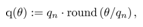 | (1) |
where θ is an input value to be quantized, and  is the quantization interval, and the function
  is the rounding function to the nearest integer. For example, Fig. 1 illustrates the quantization of
  by the quantizer,
  , with
 . Let us define a time when the quantizer output changes as
 . In this paper we call the time,
  , the interrupt time. Hence
  shows the nest interrupt time. Note that
  for all k is NOT constant. Introduce the notation to distinguish a quantized value,
  , from an original value,
  , at
, at  by
by .
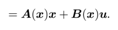
. | Figure 1. Comparison of the linear relation, y=x, with the quantizer output, q(y), in this case of qn=1 |
3. Discretization of Simple Nonlinear System by Lebesgue Sampling
In this section, in order to see through the discretization method with Lebesgue sampling, a simple nonlinear system | (2) |
is discretized by the discretization method. The following rearrangement of  can hold in general by using the chain rule.
 | (3) |
Substituting (3) into (2) yields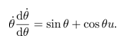 | (4) |
Suppose input of this system during the interval from  and
and ,
,  be constant. Integrating both term of (4)
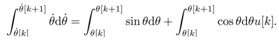 | (5) |
Rearranging (5), we have | (6) |
 | (7) |
where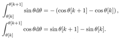 Introducing a new input,
  , the present input to (7) can be rewritten by
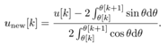 | (8) |
Hence (7) comes to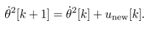 (9)Any controller will be designed for the above linear discrete formulation (9).
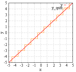
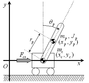 | Figure 2. The schematic figure of a cart-pendulum model.  and and  show the angle of the pendulum, the center of gravity (CoG) of the pendulum, and the CoG of the cart, respectively show the angle of the pendulum, the center of gravity (CoG) of the pendulum, and the CoG of the cart, respectively |
4. Discretization of Simple Nonlinear System by Lebesgue Sampling
A cart-pendulum system in Fig. 2 is used as a plant to be controlled in this paper. Its physical parameters and variables are shown in Table 1. The equations of motion of the cart-pendulum system are given by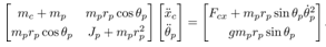 | (10) |
The following equation of motion of only the pendulum can be extracted from (10).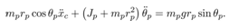 | (11) |
Table 1. Physical parameters and variables of the cart-pendulum
 |
| |
|
The acceleration of the cart,  is regarded as the input to the pendulum system (11).
 | (12) |
The following rearrangement of the angular acceleration,  can hold in general.
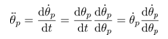 | (13) |
Substituting (13) into (12) yields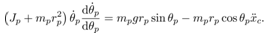 | (14) |
Suppose the acceleration of the cart during the interval from  and
and  be constant. Integrating both term of (14),
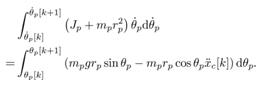 | (15) |
Rearranging (15), we have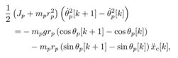 | (16) |
 | (17) |
where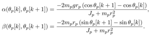 Introducing a new input,
  , the present input to (17), the cart acceleration,
  can be rewritten by
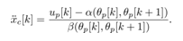 | (18) |
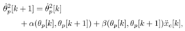
Hence (17) comes to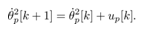 | (19) |
In (19), define the state as  and the system matrices as
  . A discrete system of the cart-pendulum system derived by Lebesgue sampling is finally given by
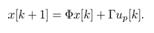 | (20) |
We're interested in a class of nonlinear systems which can be shown by the discrete system representation (20) or a time-varying discrete system representation with the same structure with (20). Unfortunately, at the moment, we cannot describe such class clearly yet. But a piston-crank model, which can present combustion engine dynamics, can be classified into this class. We also try to extend the discretization by Lebesgue sampling with multivariable case although this study just think the case only a single variable, θp, is quantized. Those issues are our ongoing works.
5. Control System Design
This paper considers a control task to realize constant-speed rotational motion for the pendulum of a cart-pendulum system. This task can be formulated by a servo control design to keep the state  of (20) be a constant desired value.To derive the following control system, we assume that the angular velocity of the pendulum,
  , can be known at each Lebesgue sampling. This implies
 | (21) |
with c=1. Of course, this assumption is not valid for the real system. Hence, this issue will be discussed later, and can be solved by combination of some numerical integration method and impulsive Luenberger observer, which is an extension of our previous method proposed by an author [7].Basically the control input,  in (20) is designed by the well-known optimal type-1 servo design[11]. Considering a quadratic cost function under the discrete system (20);
 | (22) |
the optimal state feedback control law,  is given by
 | (23) |
where P is the positive symmetric matrix as the solution of the following discrete-time Riccati equation; | (24) |
Here, define a reference value as  , and consider an augmented system as follows:
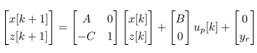 | (25) |
A state feedback control law for (25)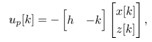 | (26) |
leads to the optimal type-1 servo controller for the closed- loop system. The feedback gain is given by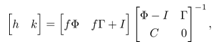 | (27) |
where f is the optimal feedback gain in (23).
6. Implementation
During an interval from  and
and  is constant and given by (26). The corresponding cart acceleration,
  is calculated by (18). Note that
  is given as a prior information, and is available for calculation of (18) because
  is an output of the quantizer, (1), and the quantization interval of (1) is known preliminarily.From (10), the cart acceleration,
  can be represented by
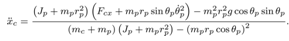 | (28) |
Therefore, once  is obtained from
 , the horizontal force applied to the real cart,
  is derived by
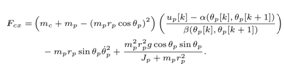 | (29) |
Note that  in (29) is continuous with respect to time, and varying even though
  and
and  are constant during the Lebesgue sampling interval, because (29) requires continuous values of
  and
and .As aforementioned, new measurement data,
  is obtained only at the interrupt time
  i.e. only when the quantizer output changes. In this sense,
  and
and  are known a priori because
  is the quantized value of the original
 . During the interrupt times, the original signals,
  and
and  cannot be measured. So (29) cannot be applied and implemented to the system directly. Hence in the following section, we propose a numerical method to solve the problem.Here we also give a remark to control the rotational direction of the pendulum. The rotational direction depends on whether define
  or
or  with the quantizer interval
6.1. Numerical Integration of Nonlinear System by Runge-Kutta Method in SDC form
To overcome the addressed issue on the implementation, the key is to introduce an impulsive Luenberger observer. This scheme is a kind of analogy in [7] and [10]. Such impulsive Luenberger observer, however, requires the mapping of the current system state to the one-step ahead state. That means a discrete system of the target nonlinear system is required. However, it is a difficult problem to obtain such discrete time system. We regard the difficulties is caused by the fact the input of the system affects to the system matrices in the case of the discretization for nonlinear systems. That is, the input must be known a priori over the interval for discretization. This requirements causes a circular reference problem in control system design because the system matrices are required a prior to design the input. In our case, on the other hand, the discrete system of the target nonlinear system is used only when the state estimation is updated posteriori, i.e, after each interrupt. The diagram of the proposed controller is shown in Fig. 3. In the following part, the detail is derived by using the cart-pendulum system as the example.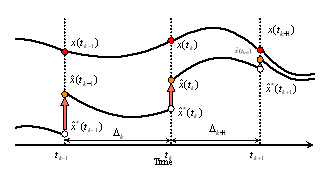 | Figure 3. The diagram of the impulsive Luenberger observer-based controller for Lebesgue sampled systems |
6.2. Non-linear System Discretization by the Runge- Kutta Method
Assume that input force u from tk to tk+1 is constant. Let a state vector of the system be 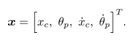 Motion equations of the system (10) can be changed the formula
 | (30) |
 | (31) |
(30) is approximated by using the Runge-Kutta method as follows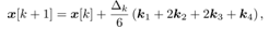 | (32) |
where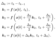 Rearranging (31) into the approximated formula, k1 is obtained as followsFor simplicity let
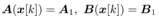
 | (33) |
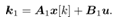
In a similar way k2 is obtained as follows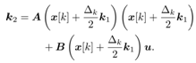 For simplicity let
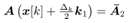 ,
, 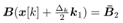
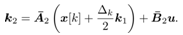 | (34) |
Rearranging (33) into (34), k2 is obtained as follows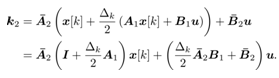 | (35) |
For simplicity let, 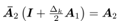 ,
, 
 | (36) |
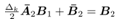
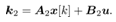
In a similar way k3,k4 are obtained as follows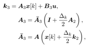 | (37) |
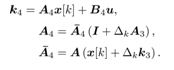 | (38) |
Thus a discretized formula of (31) can be described as follows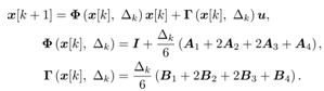 | (39) |
6.3. Impulsive Luenberger Observer
In the system if the angular velocity  can not measure then
  need to be estimated. Consequently
  is estimated by using ILO which consider the quantization of the pendulum angle. ILO is defined as follows
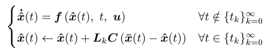 | (40) |
where  is estimated state, and
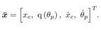 Assume that the pendulum angle
  and the cart position
  can be measured, coefficient matrix of the output equation is as follows
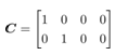 The observer gain
  can be obtained so that all eigenvalues of
 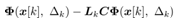 are inside the unit disc.
7. Numerical Simulation
In the following simulation the control input and the estimated states can only be updated at the quantizer transition time. The quantization interval . Setting the constant reference
  in the system (25), the angular velocity of the system is controlled to the constant velocity
 .At first simulation results with the measurement velocity
  by using the servo control law are shown. It is shown that what the quantization interval
  influence the simulation results by comparing each result with,
  and
and  .Next simulation results with only the cart position
  and the quantized pendulum angle
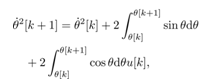
  are show. In these results the other states is estimated by using ILO (40) with the discrete system (39). The scheme of the presented control system is shown in Fig. 4.
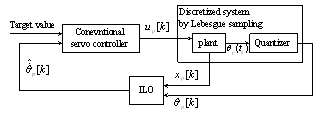 | Figure 4. Scheme of the presented control system. Observable states are the quantized pendulum angle  and continuous cart position and continuous cart position  where where  is a time when the quantizer output changes. From the observable states, we estimate is a time when the quantizer output changes. From the observable states, we estimate  by Impulsive Luenberger observer (ILO). From estimated state by Impulsive Luenberger observer (ILO). From estimated state  and target value, control input and target value, control input  is determined by a conventional servo controller. is determined by a conventional servo controller. |
7.1. Angular Velocity Control with the Measurement 
In this simulation integral calculation function is rkf45() with MaTX Windows9x/ME/NT/2000/XP(Visual C++ 2005) version 5.3.37. Step size for rkf45() is10-5. Initial condition of the pendulum angle is , the pendulum velocity is,
  otherwise 0. Weight matrices are set to
  and
and  for
for  .
.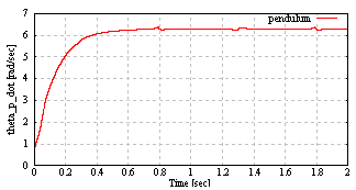 | Figure 5. The pendulum angular velocity of the cart pendulum |
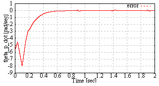
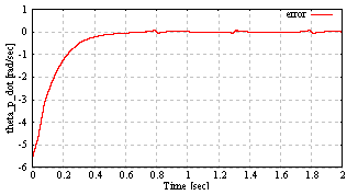 | Figure 6. The pendulum angular velocity error from constant reference  rad/sec rad/sec |
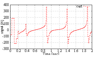
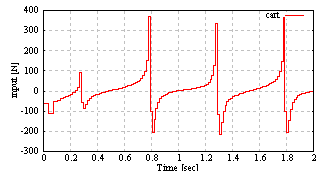 | Figure 7. The input to the cart |
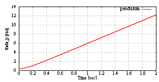 | Figure 8. The pendulum angle of the cart pendulum |
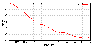 | Figure 9. The cart position of the cart pendulum |
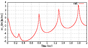 | Figure 10. The cart velocity of the cart pendulum |
From Fig. 5 and Fig. 6, the pendulum velocity  achieve the constant reference
  rad/sec. From Fig. 8, the pendulum angle monotonic increase by the pendulum velocity which achieve the constant reference. From Fig. 7, the input force to the cart updates at the quantizer transition time. From Fig. 9 and Fig. 10, the cart position and speed change with the input force which designed the above.Next, it is shown that what the quantization interval qn influence the simulation results by comparing each result with
 ,
,  and
and  . In these results, simulation conditions are the same as the above simulation without the quantization interval qn. Some simulation results are shown as follows.
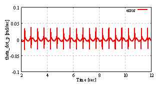 | Figure 11. The pendulum angular velocity steady error from constant reference  rad/sec with the quantization interval rad/sec with the quantization interval . In this result, simulation conditions are the same as the above simulation without qn . In this result, simulation conditions are the same as the above simulation without qn |
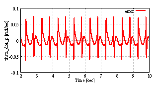 | Figure 12. The pendulum angular velocity steady error from constant reference  rad/sec with the quantization interval rad/sec with the quantization interval . In this result, simulation conditions are the same as the above simulation . In this result, simulation conditions are the same as the above simulation |
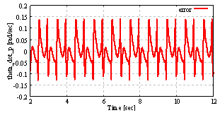 | Figure 13. The pendulum angular velocity steady error from constant reference  rad/sec with the quantization interval rad/sec with the quantization interval . In this result, simulation conditions are the same as the above simulation without qn . In this result, simulation conditions are the same as the above simulation without qn |
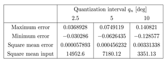
Table 2. The influence of qn with
 , ,
 and and

 |
| |
|
From Fig. 11 to Fig. 13 and Table 2, the steady error from the constant reference with shorter quantization interval is less than the steady error with larger quantization interval. In these results, square mean input of the system increase by denominator of (29). The denominator has . This term take a small value with shorter quantization interval qn.
7.2. Angular Velocity Control with ILO
In this simulation integral calculation function is rkf45() with MaTX Windows9x/ME/NT/2000/XP(Visual C++ 2005) version 5.3.37. Step size for rkf45() is . Initial condition of the pendulum angle is
 , the pendulum velocity is
 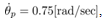 otherwise 0. Weight matrices are set to
  and
and 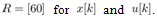 The observer gain Lk is designed discrete-time linear quadratic regulator with controllable pair
 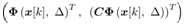 . Weight matrices are set to
 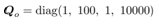 and
and  and the correction term.
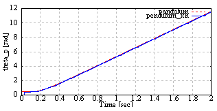
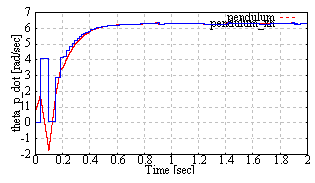 | Figure 14. The pendulum angular velocity of the cart pendulum with ILO. Red dashed line is the pendulum angular velocity . Blue solid line is the estimated pendulum angular velocity by ILO . Blue solid line is the estimated pendulum angular velocity by ILO |
 | Figure 15. The pendulum angular velocity error from constant reference  rad/sec with ILO rad/sec with ILO |
 | Figure 16. The input to the cart |
 | Figure 17. The pendulum angle of the cart pendulum with ILO |
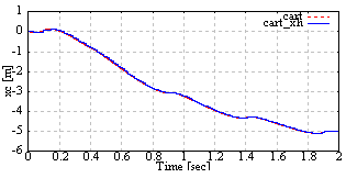 | Figure 18. The cart position of the cart pendulum with ILO. Red dashed line is the cart position. Blue solid line is the estimated the cart position by ILO |
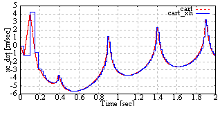 | Figure 19. The cart velocity of the cart pendulum with ILO. Red dashed line is the cart speed. Blue solid line is the estimated cart speed by ILO |
From Fig. 14 and Fig. 15, the pendulum velocity  achieve the constant reference
  rad/sec. From Fig. 14 to Fig. 19, the input force and estimated states are updated at the quantizer transition time. The estimated states achieve the real states.
8. Conclusions
In this paper, first of all, a discretization with Lebesgue sampling has been considered for a type of nonlinear system such as a cart-pendulum system. For example the cart-pendulum system is converted into the corresponding discrete system (20), which is a time-invariant linear system, by the proposed method. Hence many current control design schemes can be applied to the discrete system. On the other hand, the implementation of the controller is a crucial problem, and to overcome this problem, in this paper, an impulsive Luenberger observer has been introduced. This observer requires basically the mapping the current state to the one-step ahead state of the nonlinear system, and then a numerical integration method based on Runge-Kutta has been also derived to give such mapping. Hence the implemented controller is given by the combination of the impulsive Luenberger observer and the numerical integration method. With the controller, the output of the closed-loop system is controlled to be a desired value even though the controller works only when the quantization occurrs. The numerical simulation shows the effectiveness of the proposed system. As future works, we're now interested in the class of nonlinear systems to which the proposed system can be applied. A combustion engine piston-crank model might be an example.
References
| [1] | K. J. Åström, K. Johan and B. Wittenmark, "Computer-controlled systems. third edition", Prentice Hall, 1997. |
| [2] | K. J. Åström and B. M. Bernhardsson, "Comparison of Riemann and Lebesgue sampling for first order stochastic systems", In Proceeding of the 41th IEEE Conference on Decision and Control, Las Vegas, Nevada USA, December 2002, pp. 2011-2016. |
| [3] | K. E. Årzén, "A simple event-based PID controller", In Proceeding of the 14th IFAC World Congress, Beijin, China, 1999. |
| [4] | N. Marchand, "Stabilization of Lebesgue sampled systems with bounded controls: the chain of integrators case", In Proceedings of the 17th IFAC World Congress, Seoul, Korea, 2008, pp. 10265-10270. |
| [5] | Y. K. Xu and X. R. Cao, "Time Aggregation Based Optimal Control and Lebesgue Sampling", In Proceedings of the 46th IEEE Conference on Decision and Control, New Orleans, LA, USA, December 2007, pp. 5904-5909. |
| [6] | J. Sur and B. Paden, "Observers for Linear Systems with Quantized Outputs", In Proceedings of the American Control Conference, Albuquerque, New Mexico, 1997, pp. 3012-3016. |
| [7] | M. Iwase, S. Katohno and T. Sadahiro, "Stabilizing Control for Linear Systems with Low Resolution Sensors", 18th IEEE International Conference on Control Applications Part of 2009 IEEE Multiconference on Systems and Control, Saint Petersburg, Russia, July 8-10, 2009, pp. 1105-1009. |
| [8] | Nicola Elia and Sanjoy K. Mitter, "Stabilization of Linear Systems With Limited Information", IEEE Transactions on automatic control, Vol.46, No.9, 2001, pp. 1384-1400. |
| [9] | Tomohisa Hayakawa, Hideaki Ishii, Koji Tsumura, "Adaptive quantized control for linear uncertain discrete-time systems", Automatica, Vol.45, 2009, pp. 692-700. |
| [10] | Luis A. Montestruque and Panos J. Antsaklis, "On the Model-Based Control of Networked Systems", Automatica, vol. 30, no. 10, pp. 1837-1843 (2003) |
| [11] | T. Mita, "Optimal Digital Feedback Control Systems Counting Computation Time of Control Laws", IEEE Transactions on Automatic Control, AC-30-6, 1984, pp. 542-548. |
 Abstract
 Reference
 Full-Text PDF
 Full-Text HTML