1. Introduction

From ancient times to the modern day, assembly lines (ALs) have been modified as long as the long-term optimal design of the lines has surely been the most important milestone in the manufacturing process. Whereas designer of ALs (mostly) deal with many assembly tasks (around 400 tasks in a typical car ALs) and some critical limitations in design, the optimal solution can be achieved via a variety of heuristic ideas that must be massively computerized. Most of the work related to ALs concentrates on the assembly-line balancing (ALB) problem. The ALB problem deals with the assignment of the tasks (as duties) among workstations (or operators) so that the precedence relations are not violated, the total time for tasks in each workstation does not exceed the cycle time and a given objective function is considered to be optimized. The ALB problem falls into the NP-hard class of combinatorial optimization problems[1]. If there are n tasks and r preference constraints, then there are n!/2r possible task sequences[2]. Therefore, it can be time consuming for optimum-seeking methods to gain an optimal solution within this extremely large search space for some manufacturing operations, such as car assembly lines with more than 100 workstations.

Despite the vast search space, many studies have tried to solve the ALB problem using optimum-seeking methods, such as linear programming [e.g. 3], integer programming [e.g. 4], dynamic programming [e.g. 5] and branch- and- bound approaches [e.g. 6]. However, none of these methods has proven to be of practical use for large assembly lines due to their computational inefficiency. Hence, the next research efforts have been directed towards the development of heuristics [e.g. 7, 8] and meta-heuristics such as simulated annealing [e.g. 9], tabu search [e.g. 10] and genetic algorithms [e.g. 11].

Due to the complexity of the ALB problem, a growing number of researchers have employed genetic algorithms (GAs), and most industrial engineers also use them to optimize problems which are difficult to find an optimal solution for in a reasonable time. GAs provides an alternative to traditional optimization techniques by using directed random searches to locate optimum solutions in complex search spaces. Hence, because of the popularity of GAs’ application to the ALB problem, some papers exist which review the subject, including Dimopoulos and Zalzala[12], Scholl and Becker[13] and Tasan and Tunali[14] have all tried to modify GA using modified selection techniques, individual representation, crossover techniques etc. in order to improve the algorithms.

As having different priorities and objectives that GAs are trying to optimize as fitness functions, the ALB problem can be classified into some classes with different objectives. Additionally, the GAs’ setting in chromosomes representations, initial population, and operation mechanisms were considered by GA designers to be like challenge and benchmarking.

1.1. ALB Problem Classes and their Objectives

Before making any decisions about assembly line design, the ALB problem must be classified according to the objectives and what needs to be developed. Figure 1 illustrates the classification of ALBP based on the objective function and problem structure[2,13,15-16].

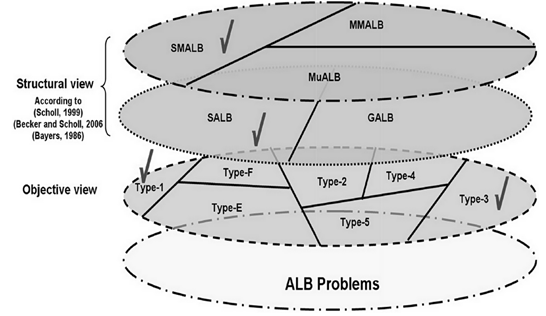Figure 1. Classification of assembly line balancing problems and our research boundaries

Scholl[16] has defined several versions of the ALB problem which have arisen by varying the objective function. Type-F is an objective-independent problem, which is to establish whether or not a feasible line balance exists for a given combination of n (number of workstations) and c (cycle time). Type-1 and Type-2 have a dual relationship; the first one tries to minimize the number of workstations for a given cycle time, and the second one tries to minimize the cycle time for a given number of workstations. Type-E is the most general problem version, which tries to maximize the line efficiency by simultaneously minimizing the cycle time and the number of workstations. Finally, Kim et al.[15] has explained that Type-3, 4 and 5 correspond to the maximization of workload smoothness, the maximization of work relatedness and multiple objectives with Type-3 and Type-4, respectively.

Based on the problem structure, ALB problems can be classified into two groups. While Becker and Scholl[16-17] have categorized that the first group includes single-model assembly-line balancing (SMALB), multi-model assembly-line balancing (MuMALB), and mixed-model assembly-line balancing (MMALB), the second group illustrated by Baybars[2], includes simple assembly-line balancing (SALB) and general assembly-line balancing (GALB). The SMALB problem involves only one product. The MuMALB problem involves more than one product produced in batches. The MMALB problem refers to assembly lines which are capable of producing a variety of similar product models simultaneously and continuously (not in batches). Additionally, the SALB problem, the simplest version of the ALBP and the special version of the SMALB problem, involves the production of only one product, where the assembly line has features such as a paced line with a fixed cycle time, deterministic independent processing times, no assignment restrictions, serial layout, one-sided workstations, equally equipped workstations and fixed-rate launching[14]. The GALB problem includes all of the problems that are not SALB, such as the balancing of mixed model, parallel, U-shaped and two-sided lines with stochastic dependent processing times; thereby, more realistic ALBPs can be formulated and solved.

Due to setting up expenditure, minimizing the number of workstations is frequently important than other criteria and, on the other side, the utility improvement of each workstation in terms of balancing the job among workstations in order to reduce the total idle time in manufacturing, is considerably more important. As a consequence, in this paper, as shown by the tickets in Figure 1, a combination of Type-1 and Type-3 based on objective, and; SMALB and SALB based on problem structure is considered and used.

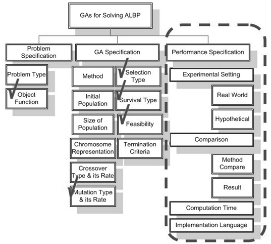Figure 2. GAs Parameters and setting for ALBPs- sources:[14]

Depending on the problem to be solved by GAs, some GA parameters and structures can be influenced. As Tasan and Tunali[14] mentioned in their paper, they have reviewed the active literature based on specifications of problem, GA and performance. As seen in Figure 2, problem specifications contain the main features of the problems studied, GA specifications summarize information about the GA methods developed, initialization of the population, chromosome (individual) representation, fitness function, genetic operators, selection and survival schemes (elitism techniques), feasibility issues, and termination criteria (final conditions that specify the end of iteration in GA)- and finally, performance specifications include information about the data sets used to test GA, other solution methods to, which the performance of GA was compared, the computation time and the implementation language.

In[14], the authors have surveyed a lot of researchers’ work that each has introduced and modified the GA for the ALB problem. Some of them worked on chromosome representation[e.g. 18,19-20]; some of them have presented modified GAs on fitness function as the basis of objective function[e.g. 11, 21]. Some of the customized crossover operators utilized include the modified bin-packing crossover (modified BPCX)[11], the modified partially mapped crossover (modified PMX)[22], the heuristic structural cro- ssover (HSX)[15], the informed order-based crossover[23], and the order crossover[19].

Tasan and Tunali[14] have reviewed the published literature based on the experimental settings in which the proposed GAs have been implemented, the other solution methods to which the GAs performance has been compared, the computation time required and, finally, the implementation language employed. However their paper has not tried to compare the performances of the reviewed GAs; it only presents the findings of the comparative studies reported in each work.

Genetic selection operation is a vital aim to find suitable parents to reproduce offspring and make a new population. The initial step always starts with a simple question “How important and influential is it that the selection of parent mechanism depends on similarities and diversities between parents”. Based the literature, maintaining the population diverted on a cellular structure called cellular automaton (CA), was first introduced by Manderick and Spiessen[24]. They presented a cellular automata genetic algorithm (CAGA) as a kind of decentralized GA in which the population is arranged in a grid (usually two dimensions). CAGAs have been successfully implemented on a parallel platform used as a computational machine[25] and have also been used for optimization and simulation problems[26]. then Cao and Wu[27] firstly brought the hamming distance idea to CAGA in order to make desirable neighborhoods in CAGA. The individuals in the population were mapped onto a CA to make the locality and neighborhood. The mapping was based on the individuals' fitness and the hamming distances between individuals. The selection of individuals was control based on the structure of the CA, to avoid the fast population diversity loss and improve the convergence performance during the genetic search. The effectiveness of the CAGA was illustrated with two typical mechanical design optimization problems (Cao and Wu, 1998). Cheshmehgaz et al.[28] have employed the proposed CAGA to solve multi-model optimization problem, channel assignment problem in cellular mobile networks, the graph-coloring problem. The work has shown the effectiveness of CAGA.

In this paper, the grid (cellular) structure for the GA’s population is used that makes the GA’s selection operation restricted to find a mat for each individual. The structure can define a local selection for individuals of the population, so that individuals must be arranged on nodes of the grid (and sometimes rearranged in fixed iterations) and each arranged individual in the node can only match (do a crossover) with its neighbor’s individuals (in neighbor nodes). The arrangement can be done on minimum hamming distance and maximum hamming distance value based upon its neighbors; and with regards to combination of it. Different kinds of neighbor definition are compared for an assembly line balancing case study with 83 tasks. Also, new mechanisms for mutation technique, objective function as fitness function, feasibility and survival type are modified and used.

The paper is organized as follows. In section 2, the typical GA and some structural frameworks used are presented and the grid structure applied for making the GA’s population structure and for defining neighborhoods is explained and the cellular genetic algorithm (CGA) family is presented. Some individuals’ arrangement and rearrangement techniques on the hamming distance basis are performed on a grid structure in order to make the hamming distance cellular GA family in section 3. In section 4, all kinds of arrangement mechanisms are tested and compared with the typical (conventional) genetic algorithm by using one large-size benchmark data set from Scholl[29]: data of assembly-line balancing problems.

2. Typical Genetic Algorithms for ALB

The structure of typical GA (TGA) is explained below as it performs one generation initial population, crossover and mutation operation in iteration.

Generate initial population

Repeat

Choose two individuals as parents for recombination

Apply crossover with R_c probability

Apply mutation with R_m probability

Replace parents with offspring

Until stopping condition is reached

Take the best chromosome of the population as the solution

GA specification is an initial step. Following subsections introduce task-based representation, initial population and crossover operation as long as new fitness function and mutation technique are introduced.

2.1. Representation

Sabuncuoglu et al.[19] has introduced task-based representation (TBR) where each task is represented by a number that is placed on a string (i.e. individual) with the string size equal to the number of tasks. The tasks are ordered by the individual relative to their order of processing. The tasks are allocated to workstations so that the sum of the task times in each station does not exceed the cycle time. This coding scheme is demonstrated in Figure 3 through a 7-task problem example as follows.

Example: we have seven tasks with own times shown in Figure 3.a, the precedence graph (matrix) are presented in Figure 3.b and the cycle time is equal to 20. Figure 3.c illustrates a string with an order of tasks that means tasks 1, task3 and task 2 are assigned to workstation 1, tasks 4, 5 and 6 are assigned to workstation 2 and finally task 7 is allocated to workstation 3. Figure 3.d shows another configuration for the task balancing equaled with the string representation that is illustrated in Figure 3.e.

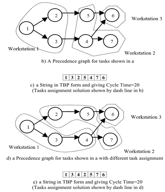Figure 3. An example shows Task-Base Representation for two different optimum solutions

2.2. Objectives and Fitness Function Definition

There are many solutions for ALB but a few of them are better than others based on some objectives. However, the important objective of the ALB problem is to minimize the number of workstations but, in practical view, the balancing algorithm should also balance the total idle times among workstations too and provide a smooth balanced solution. In the previous example, the first configuration of task balancing, Figure 3.b, needs 3 workstations. The first workstation has tasks with total time: 5+5+9=19. The second workstation with total task time: 4+6+9, needs 19 units of time, and the third workstation needs 20 units of time. In the second configuration, Figure 3.d, the first workstation needs 18 units of time, the second one needs 20 and the third one needs 20 units of time. Although the total idle times for both cases is the same and equal to 2 units of time, the first configuration is more smoothly balanced based on idle time than the second.

Hence, we have defined a utility function for fitness function that consists of two objectives, i.e. minimizing the number of workstations and maximizing smoothness among workstations. The given and decision variables are introduced as follows.

Parameters:

: Number of tasks in AL (a given variable)

: Number of needed workstations (a decision variable)

: Task identity

: Workstation identity

: A binary matrix where its rows indicate the tasks and its columns indicate the workstations: ’s value is 1 or 0. The value of 1 means that task is assigned to workstation numberand 0 means not (a decision variable)

: time (units of time) (a given variable)

: Cycle time in AL(a given variable)

: Total time the workstation is busy, 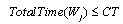(a decision variable)

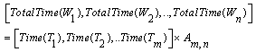(1)

: Idle time in workstation _th, (a decision variable)

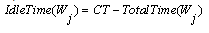(2)

Root Sum Square (RSS): the most important parameter to specify smoothness in task assignment

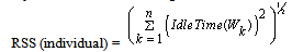(3)

Fitness function for each individual:

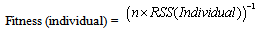(4)

Equation (1) calculates the total time for each workstation that it needs according to. Equation (2) specifies the idle time left in each workstation. Equation (3) illustrates a measure of balance and smoothness in the line by a solution and Equation (4) specifies the fitness value of a solution (used in this research).

2.3. Initial Population

The initial population is generated randomly assuring feasibility according to precedence relations. So, all individuals in the population in all generational steps will be feasible.

2.4. Crossover Technique

The two parents that are selected are cut at two random cut-points. The offspring takes the same genes outside the cut-points at the same location as its parent and the genes in between the cut-points are scrambled according to the order that they have in the other parent. Sabuncuoglu et al.[19] presented the applicable crossover technique that we follow. It is demonstrated in Figure 4. The major reason that makes the crossover operator important is that it assures feasibility of the offspring. Since both parents are feasible, both children must also be feasible. Keeping a feasible population is a key to the ALB problem since preserving feasibility drastically reduces computational effort.

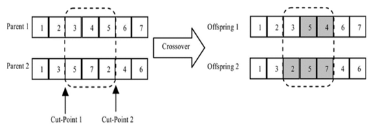Figure 4. The crossover operation (gained from Sabuncuoglu et al., 2000)

2.5. Mutation Technique

In the mutation operation, a cut-point is randomly selected and the gene (bit) in this point is replaced with next gene (right-side) if it is possible (according to precedence limitations) and then all following genes will be exchanged to right-side gen as the same till there is no possibility to exchange. Figure 5 shows one mutation in the individual shown in Figure 3.e. As it is obvious, due to feasibility, gene 4 can be replaced with gene 2 and then with 5 till it cannot be exchanged.

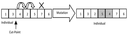Figure 5. The mutation operation

Figure 6. A 2-dimensional grid (cellular) structure with 3 nodes (cells) with different radius (1 and 2) and their neighbours

3. Cellular-Rearranging of Population

3.1. Cellular (grid) Structure

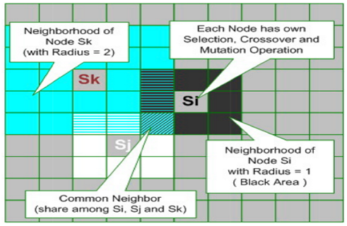
The cellular structure (CS) used in this paper is a simplified version of cellular automaton (CA). CA is a collection of cells (nodes) on a grid of a specified shape that evolves through a number of discrete time steps according to a set of rules based on the states of neighboring cells. The rules are then applied iteratively for as many time steps as desired. Von Neumann is one of the first people to consider such a model, and incorporated a cellular model into his ‘universal constructor’ Cellular automata were studied in the early 1950s as a possible model for biological systems[30]. In this paper terminology, a CS comprises three components: which is explained below.

● N: size of CS (for instance, =10 means a grid with 10*10 nodes – Figure 6 shows a 10*10 CS).

● R: radius of neighborhoods (figure 6 shows the two different radiuses with 1 and 2 – but in one CS, a unique radius amount must be used).

● O: a set of rules in each node and can be done simultaneously and separately.

The rules specify the states of nodes in the next time step. The state of node can be Boolean as active or inactive, or be a digit number, or even be binary strings. Let show the state of a node with location in row and column in CS at time and is a rule function that depends on the values of all nodes around node and the neighbourhood with radiusand one can calculate the value of the node in the next time step. Equation (5) illustrates that is calculated by function which depends on all values of neighbors in the previous time step.

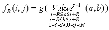(5)

The rules for GA used with CS include genetic selection, crossover and mutation operations that can be done concurrently in all nodes. One extra operation in nodes is ‘replacement’ that makes a new population by replacing new ones with olds and they must be done only after finishing one run of all genetic operations in all nodes. In the next subsection, the proposed genetic rule is going to be defined and presented.

3.2. Cellular Genetic Algorithms (CGA)

Sivanandam and Deepa[31] have classified GAs into five groups: simple GA, parallel & distributed GA, master-slave GA, coarse grained GA, and cellular GA. In the last group, the grid or fine-grained model individuals are placed on a large doughnut-shaped (the ends wrap around) one- or two-dimensional grid, one individual per grid location. The model is also called cellular because of its similarity with cellular automata with stochastic transition rules. Fitness evaluation is done simultaneously for all individuals and selection, reproduction and mating takes place locally within a small neighborhood. In time, semi-isolated niches of genetically homogeneous individuals emerge across the grid as a result of slow individual diffusion. This phenomenon is called isolation by distance and is due to the fact that the probability of interaction of two individuals is a fast decaying function of their distance. Recently Alba and Dorronsoro[32] have surveyed all conditions in CGA as a completed survey.

The following is a conventional the cellular genetic algorithmic (and are the parameters which show the probability of performing crossover and mutation operations set by a GA designer)[31-32]:

Generate a random individual j (feasible solution)

End parallel for

While not termination condition do

For each cell j do in parallel

Evaluate individual j (fitness function calculation)

Select a neighboring individual k

Produce offspring from j and k with probability

Mutate j with probability

Assign one of the best offspring to j

End parallel for

End while

In a more sophisticated view of CGAs, the new capsulated definition is presented. The capsulated definition helps to understand GAs in CS. First, the nodes must comprise two parts of information saved in the nodes in two successive time steps: and illustrate the genetic individuals (string/chromosome) at time steps and; and and are as previously defined in Section 3.1, but in two successive time steps. Secondly, the rule that calculating the values of the nodes comprises all genetic operation- selection, crossover and mutation - at once. The following pseudo codes show the modified rule function components and their order according to the genetic algorithms steps.

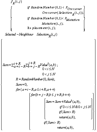
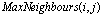
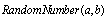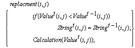
function generates a random number between a and b, and works by a local selection mechanism and neighborhood; radius reveals a location of the neighbor which has already been selected for crossover operation in node. Fitness proportionate selection, also known as the roulette-wheel selection method, is employed by operation[33]. The crossover and mutation operations that are mentioned in the pseudo code work as they are designed in TGA locally (see Section 2).

An issue in CGA is elitism strategy which means the best individuals in the old population should survive to the next population. Due to local selection in CGA, it cannot apply the strategy directly. In the final steps of CGA, replacement is considered and the best string (individual) among offspring based on fitness value would be a substitute for the old individual in node. The function replaces the old value in the node with the best value gained from the last two time steps (see pseudo code following). And the value of individual fitness that is saved as in the node must be calculated again by.

In this paper, there are also some modifications in CGA as follows.

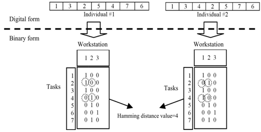Figure 7. Transfer process to binary form and hamming distance calculation

3.3. Hamming distance (HD)

Making the selection operation restricted is well-known strategy to prevent genetic drifting[34]. The grid structure can be usefully used to make the restriction[32]. In order to have a variety mates to be selected by individuals, in this research, the hamming distance parameter is considered specifying the similarity value among individuals. Each individual might be transferred to binary form as the assignment matrix (see Figure 7 – the columns specify the workstations number and the rows specify the tasks number in the assignment matrix, and the ‘1’ or ‘0’ symbol in each element illustrates which task is or is not assigned to which workstation) and then the value of the hamming distance can be calculated by counting the different 0s and 1s in genotype of individuals. Figure 7 illustrates the transfer process from phenotype (digital) form (task-based representation) to genotype (binary) form (assignment matrix) and the concept of similarity between individuals by using the hamming distance value. The example (in Figure 7) shows the value of between individual #1 and #2 is 4 or, in another definition, .

It is assumed that if mates are similar (or dissimilar) to each other they would be better parents to make offspring. To put this idea to the test, some steps in CGA need to be modified. The next subsection shows a new change in CGA in the new step, ‘cellular rearrangement’ and it seems to work like pre-processing before doing any genetic operation in each generation or frequently.

3.4. Rearrangements and CGA family

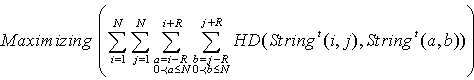
Some kinds of arrangement are selected to locate the individual on a grid’s nodes. By the arrangements we try to test the effectiveness of making the neighborhood. For instance, what if one individual could have a greater chance to have crossover with another individual that is so similar to or different to it.

In this research, three kinds of arrangements techniques are used: max-hamming distance, min-hamming distance and max-min-hamming distance, and then all are mixed with CGA as an added step and make the CGA family (Figure 8 shows the new framework of the CGA family).

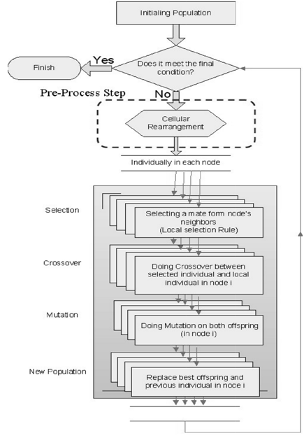Figure 8. Flowchart Abstract of CGA Family

Max-Hamming distance cellular genetic algorithm (MaxHCGA): it makes a variety of dissimilarities between the neighboring nodes. Actually, in the max-hamming distance rearrangement, the objective in individual arrangements can be formulated by (6).

(6)

To make the simplest and most heuristic way to follow the objective, all steps in MaxHCGA are the same as CGA steps but only one step must be added: cellular rearrangement. After making the initial population, according to Section 2.3, one individual from the population is randomly chosen. The chosen individual is allocated into the node called pivot and then for all empty neighbors of the pivot, the rearrangement method continues to find individuals from the rest of the population that have the maximum hamming distance value with the individual in the pivot. The rearrangement method would work for all nodes that have an individual in and at least one empty neighbor. The rearrangement can be repeated each generation or different frequently. In this paper, the rearrangement is performed before each genetic generation to realize the effectiveness of the arrangement.

Min-Hamming distance cellular genetic algorithm (MinHCGA): as it is compared with MaxHCGA, only the rearrangement method’s objective should be changed. In spite of using maximum hamming distance value, MinHCGA uses minimum hamming distance value for the rearrangement method. As a consequence, all individuals have more chance to meet individual who are more similar to. The objective considered in the rearrangement is formulated by (7).

(7)

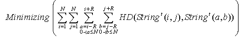
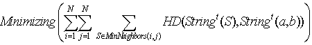
Max-Min-Hamming distance cellular genetic algorithm (MMHCGA): a combination of rearrangements of Max-HCGA and Min-HCGA makes MMHCGA which means that, alternately, Max-HCGA rearrangement and Min-HCGA rearrangement can be used. Let represent a set of all the neighbors around node that are supposed to have maximum hamming distance valued with the individual allocated in node, and 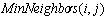embody a set of the neighbors who are supposed to have minimum hamming distance value with the individual in node. The objective of rearrangement in MMHCGA can be presented by two formulations (8) and (8).

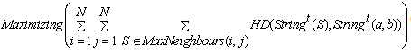(8)

(9)

For example, Figure 9 illustrates four stages of such a simple rearrangement method in MMHCGA explained by formulas (8) and (9). First, one node in CA as a pivot cell and one individual as a pivot individual randomly are chosen and the individual will be assigned to the cell. The arrangements will be continued for the pivot’s empty neighbors as following. For the pivot cell’s neighbors- the nodes in black in Figure 9.a- the maximum hamming distance value is considered, and for the others –the nodes in white –the minimum hamming distance value is used. To continue, in Figure 9.b, one of the grid’s none-empty nodes is randomly chosen, and the rearrangement is repeated until all nodes have one individual.

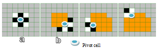Figure 9. Initial four steps of MMHCGA Rearrangement.

4. Simulation and Results

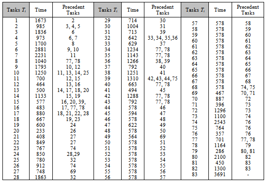
To analyse the CGA algorithms family, a case with 83 assembly tasks were selected [from 29]. The given cycle time for all workstations is 5000 units of time. To make the results quite clear and also finding the differences between the CGA family and typical (ordinary non-cellular) GA, the following parameters values were fixed, but the values could be changed to different values also.

The time of each task has been shown in Table 1. Each algorithm executed from the initial population created randomly, by 100 executions with 300 iterations in each. The best individual and the worst individual (based on fitness value) in new populations generated by the algorithms, were recorded at the end of iterations of 10, 20, 30… and 300. And the average fitness value at the end of the iterations for all CGA family algorithms were also calculated and recorded.

An individual that has used the minimum number of workstations and has minimal RSS (root sum square) of idle times was identified as a relative best task balancing solution here. We compared the all member of CGA family with each other and the typical GA (TGA) on these circumstances.

As the GA parameters part involved, to set the parameters for GA, the selection rule that is used is the roulette selection technique, and other parameters are fixed as follows.

Genetic parameters setting:

● Population size: 100

● Selection rule: roulette wheel selection

● Crossover rate: 0.9

● Mutation rate: 0.2

● Elitism rate: 0.05 (only for TGA)

● Iteration (reproduction of population) number: 300

● Number of Executions (for sampling): 100

As mentioned before, the best solution would be the one (set of) individual(s) that has(have) minimum number of workstation (that it needs) and minimum RSS of idle times (maximum smoothness of tasks) by giving CT=5000.

Table 1. Precedence table of the case study

Figure 10, illustrates behaviors of five considered genetic algorithms including TGA (conventional non-cellular GA) and CGA family employed for the case study. As Figure 10.a shows, MaxHCGA has best behavior in decreasing RSS of idle time average as long as the number of iterations is going up. In contrast to MaxHCGA, MinHCGA behaves in worst manner which means that there is no decline in the average of RSS that is expected as the number of iterations is increasing.

Considering the average of number of workstations, Figure 10.b illustrates that MaxHCGA notably attain a better solution compared with others (16.02 as workstations average needed).

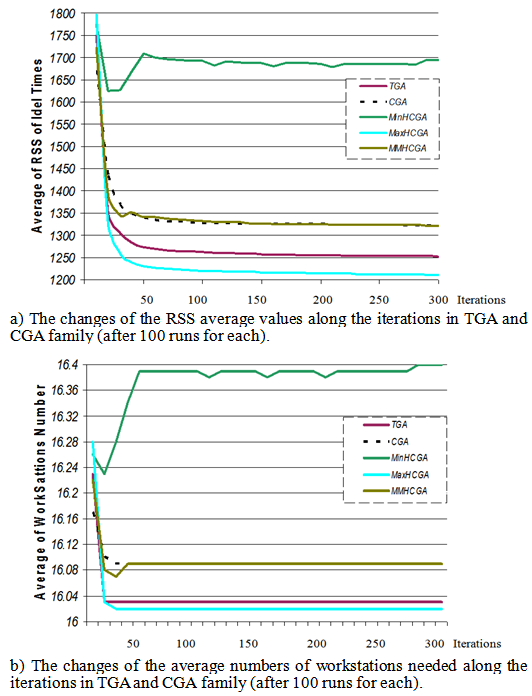Figure 10. CGS family behaviors in different iterations (on average values of RSS and needed workstations number basis)

In addition, Figure 11 shows the minimal RSS and maximal RSS of idle times, for all executions, in different iterations (for each algorithm). The values of both the parameters show that MaxHCGA works as well as it has been expected. The minimum RSS of idle times reached by MaxHCGA is about 1148.5 in the last iteration, 300 iterations (Figure11.a) and also the maximum RSS for MaxHCGA is better than others (Figure 11.b – about 2409).

Figure 12 presents the two examples of the best solutions attained by MaxHCGA and TGA at the final iteration. Each colored-row in Figure 12 is nominated as one workstation, ordered from number 1 to 16, and tasks have been marked by colored bars and the task times underneath. The idle time bars of workstations are specified in thick dash-rectangles and their values are in front.

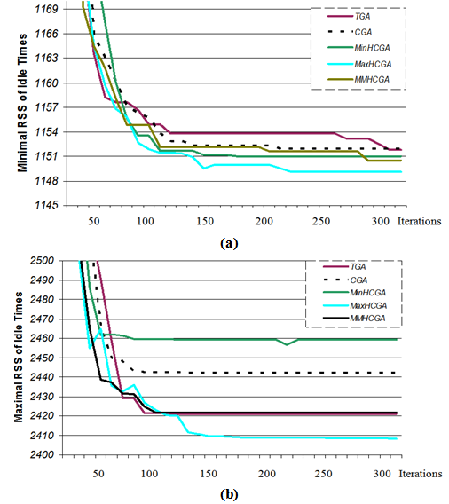Figure 11. CGS Family behaviors in different iterations (on minimum and maximum value of RSS basis)

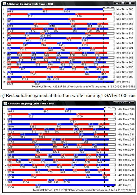Figure 12. Two best solutions of MaxHCGA and TGA by iteration 100.

In spite of TGA, MaxHCGA has found the solution with the greater smoothness level. However both solutions present the same number of workstations (equal to 16 workstations) and total idle times ( = 4293), but they have reached a different RSS of idle times as smoothness (RSS for MaxHCGA is 1149.49 and for TGA is 11.54.04). It means that MaxHCGA has found a solution which is more smoothed.

In this research, a modified cellular GA was developed to solve the single-model ALB problem comprised of Type-1, Type-3, SALB and SMALB. Some heuristic rearrangement techniques based on hamming distance values were utilized and then the CGA family was defined. We showed that each member of the CGA family initiates a chance to individuals put on cells to find a particular mate from their neighbors (by a local selection mechanism), and then tries to do all genetic operations: crossover, mutation and replacement, locally and individually. With the aim of the rearrangements techniques, the concept of exploration/exploitation has been sharpened and examined for the ALB problem case. In the ALB case, the similarity between individuals calculated by hamming distance value illustrates how much similarity exists between task assignments to the workstations proposed by individuals. The main point of this paper showed how much the similarity and dissimilarity between parents is useful for making offspring for the next generation. TGA as conventional non-cellular GA, CGA, MinHCGA, MaxHCGA, MaxMin- HCGA were all put on a test given by a test case, and then the comparison results show how much the similarity and dissimilarity in selection operations have been influenced. We concluded that MaxHCGA mostly achieves the solutions that have the minimal root sum square of idle times with comparing to other CGA family members and TGA.

5. Conclusions

Although two conventional criteria; minimum workstations and idle times, were considered here, other pragmatic criteria such as material handling constraints, resource limitations, human factors and multiple or mixed-model assembly manufacturing issues can be considered as further research directions.