Peter Matisko, Vladimír Havlena
Czech Technical University in Prague, Faculty of Electrical Engineering Department of Control Engineering
Correspondence to: Peter Matisko, Czech Technical University in Prague, Faculty of Electrical Engineering Department of Control Engineering.
| Email: |  |
Copyright © 2012 Scientific & Academic Publishing. All Rights Reserved.
Abstract
The performance of Kalman filter depends directly on the noise covariances, which are usually not known and need to be estimated. Several estimation algorithms have been published in past decades, but the measure of estimation quality is missing. The Cramér-Rao bounds represent limitation of quality of parameter estimation that can be obtained from given data. In this article, The Cramér-Rao bounds for noise covariance estimation of linear time-invariant stochastic system will be derived. Two different linear system models will be considered. Further, the performance of earlier published methods will be discussed according to the Cramér-Rao bounds. The analogy between the Cramér-Rao bounds and the Riccati equation will be pointed out.
Keywords:
Cramér-Rao bounds, Kalman Filter, Noise covariance estimation
Cite this paper: Peter Matisko, Vladimír Havlena, Cramér-Rao Bounds for Estimation of Linear System Noise Covariances, Journal of Mechanical Engineering and Automation, Vol. 2 No. 2, 2012, pp. 6-11. doi: 10.5923/j.jmea.20120202.02.
1. Introduction1
The Cramér-Rao (CR) bounds represent a limitation of the estimation quality of unknown parameters from the given data. If the variance of the estimates reaches CR bounds, it can be stated that the estimation algorithm works optimally. In this paper, we will derive CR bounds for the estimation of noise covariances of a linear stochastic system. The noise covariances are tuning parameters of Kalman filter, and the filter performance depends on them. However, they are not known in general and hence tuning of a Kalman filter remains a challenging task. The very first methods for noise covariance estimation were published in 70s’ by Mehra,[1,2]. Recently, new methods were proposed by Odelson et al. [3] and further modified by Rajamani et al.[4,5] and Akesson et al.[6]. A maximum likelihood approach was described in[7]. In Section 5, these two approaches will be compared to the CR bounds and their performance will be discussed. In the last part of the paper, relationship between the Riccati equation and the CR bounds will be pointed out.Deriving of the noise covariance CR bounds is based on[8] and[9]. Additional information about CR bounds and Bayesian estimation can be found in[10].
2. Cramér-Rao Bounds
The task is to estimate a vector of parameters  from a set of measured data
  . The upper index N emphasizes that vector yN contains N data samples. The conditioned probability density function (pdf)
  is assumed to be known. Further, the nabla operator is defined as
 | (1) |
The Fisher information matrix (FIM)  for parameters
  is defined as
 | (2) |
where operator  is the conditioned expected value defined as
 | (3) |
Alternatively, we can define a posterior FIM (and posterior CR bounds) using joint probability  instead of the conditioned one, where
  . Probability function
  represents prior information about the parameter vector
  . Assume having an unbiased estimate of parameter vector
  obtained by an arbitrary method. When the true value of parameter vector is compared to the unbiased estimated set, the following inequality holds, [8].
 | (4) |
where  represents the Cramér-Rao bound. Inequality
  means that
  is a positive semidefinite matrix. Based on (4), the following statement can be concluded. Assuming that CR bound is reachable, any estimation algorithm working optimally (in the sense of the smallest covariance of obtained estimates), must give estimates whose variance is equal to the Cramér-Rao bound. If the CR bound is reachable, then the optimal result can be achieved by a maximum likelihood approach.Consider a scalar linear stochastic system
 | (5) |
where  and
and  represent the state and the measured output, respectively. Stochastic inputs
  and
and  are described by normal distributions
  | (6) |
Using the notation of[9], the logarithms of the conditioned probability of the state, measurements and unknown parameters can be expressed as | (7) |
The following matrices are used for FIM calculation | (8) |
 | (9) |
 | (10) |
 | (11) |
 | (12) |
 | (13) |
 | (14) |
 | (15) |
 | (16) |
Further, recursive formulas for FIM of the state and unknown parameters are defined as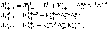 | (17) |
where 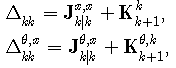 | (18) |
 | (19) |
and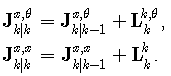 | (20) |
Initial conditions of the recursive algorithm are set as  | (21) |
where  and
and  represent prior information. If no prior probability function is known, then
  The final form of FIM of the state and parameters is
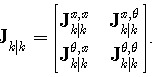 | (22) |
3. Cramér-Rao Bounds for Noise Covariances Estimation
Consider a scalar stochastic system given by (5), where  The noise sources are not correlated and are defined by (6). The probabilities used in (7) can be defined as
 | (23) |
Now, matrices (11)-(16) can be calculated using the following general integral formulas, assuming 
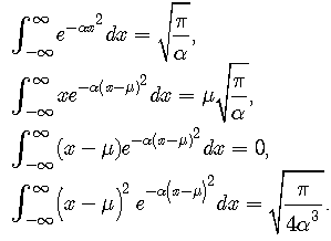 | (24) |
Further, logarithm of the Gaussian function is given by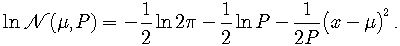 | (25) |
CR bounds of Q, R estimates are to be found, considering a scalar system with two unknown parameters. The  nabla operator, in this case, is of the form
 | (26) |
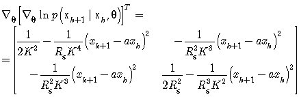
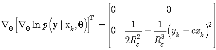
where  At the first step, the arguments of the expectation operators in (11)-(16) are calculated as follows
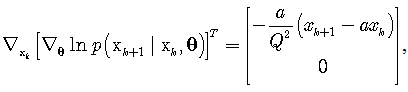 | (27) |
 | (28) |
 | (29) |
 | (30) |
Next, matrices (11)-(16) are obtained using integral formulas (24) as | (31) |
 | (32) |
 | (33) |
 | (34) |
 | (35) |
 | (36) |
It can be seen from (31)-(35) that several of the matrices are zero which significantly simplifies formula (17). In particular matrix  in (22) is zero and this fact allows us to calculate FIM for unknown covariances independently on the states. The resulting FIM can be written as
 | (37) |
where  represents the prior information about unknown parameters Q, R. If no prior information is available, it can be set to zero. From the above equations and the form of matrices in (31)-(35), it can be seen that FIM is calculated for each covariance independently. Formula for FIM is of the form
 | (38) |
where it can be assumed that  A particular closed form solution to recursive formula (38) is given by
 | (39) |
4. Cramér-Rao Bounds for a System in Innovation Form
In Section 2, a stochastic system was defined using (5). The system has two independent sources of uncertainty, the process noise and the measurement noise. It is assumed the process and the measurement noises to be normal with zero mean and covariances Q, R, respectively. In non-scalar case, variables Q, R are matrices and contain redundant information. Noise covariances represent properties of the noise sources. Considering a higher order system allows us to model the same number of noise sources as the sum of numbers of states and outputs. Matrix Q would have the same dimension as the number of states and matrix R would have a dimension equal to the number of outputs. However, from the observed output data, only the number of noise sources equal to the number of outputs can be recognized. Therefore, we can alternatively use the so-called innovation form of stochastic system that represents a minimal form,[11] or [12]. The disadvantage of such formulation comes from the fact that we loose the physical background of the noise sources and their structure. However, in many cases, we only have output data at hand and no other additional information about the stochastic inputs. In such case, the innovation form of the stochastic system can be used | (40) |
where K is a steady state Kalman gain and  is the stationary innovation process. Then
 | (41) |
The Cramér-Rao bounds for K, Rε estimation are derived using the same formulas as for the system (5). Analogously to formulas (27)-(30) we define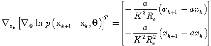 | (42) |
 | (43) |
 | (44) |
 | (45) |
The expected values are calculated using integral formulas (24). Matrices (11)-(16) are of the form | (46) |
 | (47) |
 | (48) |
 | (49) |
 | (50) |
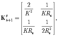
The formula for FIM calculation is of the form (37). Substituting (48) and (50) to (37) leads to the resulting formula  | (51) |
5. Comparison of the Methods for Noise Covariance Estimation
In the previous sections, we derived the CR bounds for noise covariances estimation. In this chapter, a comparison of ALS (Autoregressive least squares) method and maximum likelihood method will be presented. The ALS method, [3-5], uses the assumption that estimated autocorrelation function calculated from the finite set of data converges to the true autocorrelation function. In[7], it is shown that the assumption of fast convergence is not correct and this fact can significantly limit the quality of the estimates. In the same paper, a maximum likelihood approach is demonstrated using a simple maximum seeking method. We can compare performance of both approaches according to the CR bounds. The ALS algorithm prior setting contains the optimal Kalman filter gain and the maximum lag for autocorrelation calculation  . The ML method searches the maximum in the interval 0.1 to 10. The grid is logarithmic and contains
  points.Consider a system of the form (5) where
  ,
, 
 and
and  . The estimation algorithm uses k time samples and is repeated 300 times. Then, the resulting variance of the estimates is calculated. The dependence of the variance of the estimated Q-parameters on the number of used data samples is shown in Figure 1.
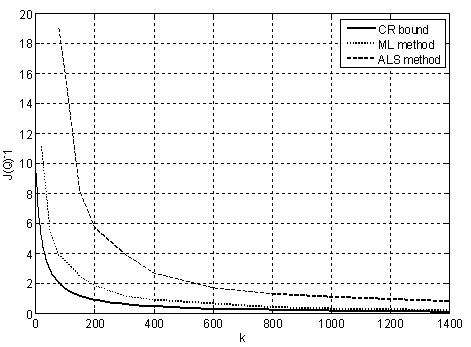 | Figure 1. Cramér-Rao bound for Q estimation and variance of estimated Q using ALS and Maximum likelihood method |
In Figure 2, an analogous result for R estimation is shown. We can state that ML method converges faster to the CR bound than ALS. ML algorithm gives better estimates in case of covariance Q than ALS even with very small sets of data (around 50 samples). 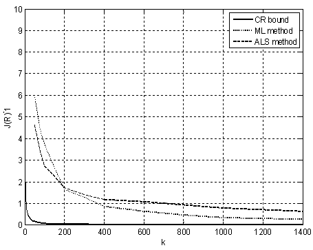 | Figure 2. Cramér-Rao bound for R estimation and variance of estimated R using ALS and Maximum likelihood method |
6. Relationship between Cramér-Rao Bounds and Riccati Equation
In this section, we will point out the relationship between Riccati equation (RE) and CR bounds. It is well known, that under some conditions, Kalman filter is optimal. It was stated in the previous section, that CR bounds represent a limit of estimation quality. Therefore, it can be expected that RE should converge to CR bounds for state estimation of a linear system. Using formulas (8)-(10) and (14), the CR bounds for state estimation can be easily obtained, Tichavský et al. (1998). We have | (52) |
Now, the recursive formula for FIM calculation, Šimandl et al. (2001), is of the form | (53) |
Using (52) we obtain resulting formula | (54) |
Riccati equation is of the form | (55) |
It can be stated, that  and
and  converge to the same matrix. Moreover, if initial values
  , then trajectories of
  and
and  are the same. This fact proves the optimality of Kalman filter. Equivalency of equations (54) and (55) is proved in Appendix .
7. Conclusions
In this paper, Cramér-Rao bounds for the noise covariance estimation were derived for two different stochastic models. From (31)-(35), it can be seen that matrices  ,
,  and
and  are zero, that means that the information between state and noise covariances is not correlated. It can be concluded that the covariances and the states can be estimated independently of each other. Another observation can be done on matrices (33) and (35). It can be seen that there is no correlation between information about the covariances. That means that CR bounds can be calculated for each covariance separately. Considering limit cases, Q converging to zero and R being arbitrary large, CR bound for Q estimation will converge to zero either. It means that there exists a method that can estimate Q up to an arbitrary level of accuracy.CR bounds can be used as a quality measure for all newly proposed estimating algorithms. We have compared a maximum likelihood approach with ALS method of Odelson et al. (2005) according to the CR bounds. Based on these examples (Figure 1 and Figure 2), it can be observed that the CR bounds for the noise covariances converge to zero relatively fast even for small sets of data (200 to 400 samples). In Section 6, we pointed out a relationship between Fisher information matrix recursive formula and Riccati equation. Equivalence of the equations is proved in Appendix 1. We concluded that this is another proof of optimality of Kalman filter.
ACKNOWLEDGEMENTS
This work was supported by the Czech Science Foundation, grant No. P103/11/1353.
Notes
1.This paper was presented at the 18th IFAC World Congress, Italy. [online]
APPENDIX
Consider two recursive equations (56) and (57) that are Fisher information matrix recursive equation and discrete Riccati equation. Both equations are equivalent and  for sufficient large k, not necessarily
  .
. | (56) |
 | (57) |
The right side of equation (56) is modified using substitution 
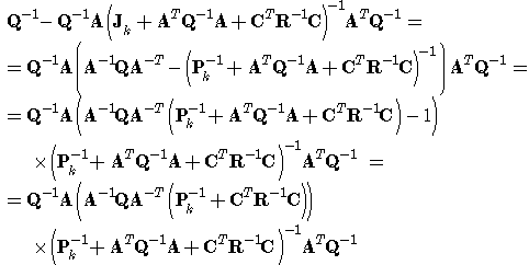 Now, both sides of the equation are inverted, so the left side is
  and the right side is of the form
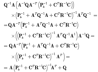 | (58) |
Further, an inversion lemma  | (59) |
will be applied on the expression  . The final formula is of the formwhich is exactly Riccati equation.
References
| [1] | Mehra R.K. (1970). On the identification of variances and adaptive Kalman filtering, IEEE Trans. on Automat. Control, AC–15, pp. 175–184. |
| [2] | Mehra R. K. (1972). Approaches to Adaptive Filtering, IEEE Trans. on Automat. Control, AC–17, pp. 693–698. |
| [3] | Odelson B. J., Rajamani M. R. and Rawlings J. B. (2005). A new autocovariance least–squares method for estimating noise covariances, Automatica. Vol. 42., pp. 303–308. |
| [4] | Rajamani M. R. and Rawlings J. B. (2008). Estimation of the disturbance structure from data using semidefinite programming and optimal weighting, Automatica, Vol. 45, pp.1–7. |
| [5] | Rajamani M. R. and Rawlings J. B. [online]http://jbrwww.che.wisc.edu/software/als |
| [6] | Akesson B. M., Jorgensen J. B., Poulsen N. K. and Jorgensen S. B. (2008). A generalized autocovariance least–squares method for Kalman filter tuning, Journal of Process control, Vol. 18, pp. 769–779. |
| [7] | Matisko P. and Havlena V. (2010). Noise covariances estimation for Kalman filter tuning. Proceedings of IFAC ALCOSP, Turkey. |
| [8] | Tichavský P., Muravchik C. H. and Nehorai A. (1998). Posterior Cramér-Rao Bounds for Discrete-Time Nonlinear Filtering. IEEE Trans. on Signal Processing. Vol. 46, pp. 1386-1396. |
| [9] | Šimandl M., Královec J. and Tichavský P. (2001). Filtering, predictive, and smoothing Cramér-Rao bounds for discrete-time nonlinear dynamic systems. Automatica. Vol. 37, pp. 1703 – 1716. |
| [10] | Candy J. V. (2009). Bayesian Signal Processing, John Wiley & Sons, Inc., USA. |
| [11] | Ljung L. (1987). System Identification, The Theory for The User. Prentice Hall, USA. |
| [12] | Kailath T., Sayed A. H. and Hassibi B. (2000). Linear Estimation. Prentice Hall, USA. |
| [13] | Anderson B. D. O. and Moore J. N. (1979). Optimal filtering, Dover Publications, USA |
| [14] | Matisko P. (2009). Estimation of covariance matrices of the noise of linear stochastic systems, Diploma thesis, Czech Technical University in Prague. |
| [15] | Matisko P. and Havlena V. (2011). Cramér-Rao bounds for estimation of linear system noise covariances, Proceedings of the 18th IFAC World Congress, Italy. |
| [16] | Papoulis A. (1991). Probability, Random Variables, and Stochastic Processes Third edition, Mc. Graw-Hill, Inc., USA. |
 Abstract
 Reference
 Full-Text PDF
 Full-text HTML