Ayan Sadhu , Sriram Narasimhan
Department of Civil and Environmental Engineering, University of Waterloo, Waterloo, N2L 3G1, Canada
Correspondence to: Ayan Sadhu , Department of Civil and Environmental Engineering, University of Waterloo, Waterloo, N2L 3G1, Canada.
| Email: |  |
Copyright © 2012 Scientific & Academic Publishing. All Rights Reserved.
Abstract
Auxiliary damping devices such as tuned mass dampers (TMD) are one of the effective means of reducing structural vibration and occupant’s discomfort of high-rise building. When tuned to resonant mode of vibration of the primary structure, an optimally tuned TMD introduces significant damping in the dynamical system, thereby reducing the overall vibration response of the structure. However, deterioration of TMD, accidental changes in the operating conditions, in-correct design forecasts, etc., leading to de-tuning in TMDs, may exhibit a significant loss in their performance. To restore optimal performance, it is necessary to quantify the de-tuning condition of the existing systems and then re-tune the TMD to its optimal state. Therefore, an adaptive and automated detection of real-time de-tuning level of the TMD is one of the key challenges in the area of structural system identification. Time series models works extremely well in capturing the key features of any data series. In the present study, output-only time series models are used to detect the de-tuning level of TMDs. The basic idea is to simulate different class of models with wide range of de-tuned levels in equivalent finite element model of the real structure and compare with its true responses to identify its unknown de-tuning level.
Keywords:
TMD, System Identification, ARMA Model, Parameter Estimation
Cite this paper:
Ayan Sadhu , Sriram Narasimhan , "Identification of De-Tuning Level of Tuned-Mass-Damper System Using Time-Series Analysis", Journal of Mechanical Engineering and Automation, Vol. 2 No. 1, 2012, pp. 1-8. doi: 10.5923/j.jmea.20120201.01.
1. Introduction
In the era of high performance flexible structures like Taipei 101, Burj Dubai, CN tower, and Petronous towers, estimation of dynamic properties, i.e., natural frequencies, damping and mode shapes, is of paramount importance. Its significance stems from the fact that such structures are liable to undergo changes over time, sustain damage, and/or get augmented by supplemental energy dissipation devices aimed at controlling their motions against wind or other disturbances. The dynamical properties are essential ingredients for the structural health monitoring. Extracting system information often needs to be accomplished exclusive of the knowledge of inputs, and is referred to as ambient system identification. Its importance is evident because in many practical civil structures like tall skyscrapers or long bridges, measurement of the excitations (wind/earthquake) can be prohibitively difficult. Outputs on the other hand can be measured relatively easily through an organized sensor network without disturbing the in-service conditions.Tall civil engineering structures are susceptible to vibrations due to their flexibility, lack of sufficient inherent damping and the wind induced excitation at such heights. Auxiliary damping devices are an effective means ofreducing structural vibration and occupant’s discomfort. Tuned mass dampers (TMD) are perhaps the most commonly used passive vibration control devices in flexible structures [1-4]. For example, Taipei 101 and its TMD are shown in Fig. 1. When tuned to the resonant mode of vibration of the primary structure, a well-tuned TMD (optimal TMD) adds significant damping in the dominant vibration modes, thereby reducing the overall vibration response of the structure. The performances of TMDs have been well studied in the literature [6-9]. De-tuning of the TMDs, resulting from several sources such as the alteration of the structural properties of the primary structure, deterioration of the TMD, in-correct design forecasts, etc., may lead to a significant loss in their performance. Therefore, the detection of the real-time de-tuning level of the TMD is one of the key challenges in the area of structural system identification [14, 15]In the present study, time series models [11, 12] are used to detect the level of de-tuning in TMDs. Since the problem is related to the output-only system identification, transfer-function noise (TFN) based input-output model is not employed, rather output-only random noise based auto-regressive moving average (ARMA) time-series models are explored. The basic idea is to simulate different class of de-tuned models based on the suitable finite element model of the real structure. Then the corresponding response time series are computed from the simulated de-tuned models and then the times series models are generated based on these responses. Upon receiving the actual or true responses of the de-tuned system, the unknown level of de-tuning in the actual system can be estimated by comparing the previously developed time series models of the simulated de-tuned systems and the experimental data.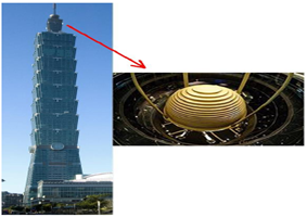 | Figure 1. Taipei 101 and its TMD (www.wikipedia.org) |
2. Basic Dynamics of TMD
In order to understand the basic dynamics of the TMD system, it is instructive to observe the equations of motion for a two-degree-of-freedom representation for the system shown in Fig. 2. The system is simply a single-degree-of-freedom (SDOF) primary system with a TMD at top.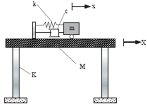 | Figure 2. DOF system with TMD at top |
The equations of motion for the system in Fig. 2 can be written as [10]: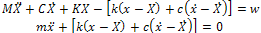 | (1) |
Where M, C, K are the mass, damping, and stiffness coefficients of the primary structure, and m, c, k are the mass, damping, and stiffness coefficients of the TMD. w is the external excitation source, which is assumed to be stationary white Gaussian for the purposes of this study. Wind excitation under normal ambient condition usually satisfies such statistical characteristics. Frequency of the primary structure (fp) and the TMD (ft) can be expressed as: | (2) |
The TMD parameters are specified by its: (a) mass ratio (µ = m/M), (b) frequency ratio (f = ft/fp), and (c) damping ratio (ξ). These quantities represent the ratio of the TMD parameters to the corresponding primary structure parameters. The optimum TMD parameters, the optimum stiffness (fopt) and damping (ξopt) are determined as a function of µ and primary structure damping ratio (ξp) using the regression expressions as described in the literature [10]. Finally, kopt and copt of TMD can be expressed as: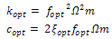 | (3) |
Where Ω is the natural frequency of the primary system to which the TMD is tuned. While designing a TMD, the optimum parameters are calculated based on above expressions. However, at a later stage, when the TMD properties get altered due to several reasons as described in the previous section, it is said as “de-tuned”. In the present study, it is assumed that the source of de-tuning is due to both the stiffness and damping of TMD. The level of de-tuning condition is quantified as:  | (4) |
Where α and β are the de-tuning parameters for stiffness and damping respectively. For example, α=1 and β =1 imply an optimally designed TMD. On the other hand, for the de-tuned system, α≠1 and β≠1.Of particular interest is the case of TMD for a general N multi-degree-of-freedom (MDOF) primary structure as shown in Fig. 3. Using the dynamical modal analysis, the equations of motion for the i-th mode when the TMD is present in the j-th floor level can be written as: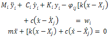 | (5) |
where, the quantities Mi, Ci, Ki, wi should be interpreted as corresponding to the i-th mode.
2.1. Numerical Illustration of a De-tuned TMD System
A 5-storey structure model with a TMD at the top floor [10] is simulated to demonstrate the basic dynamics of TMD and to present the key results for the present study. The natural frequencies of the model are 0.91, 3.37, 7.1, 10.67 and 12.71 Hz respectively. The state-space model for this system subjected to an external disturbance vector, w is given by: | (6) |
Here, the vector x is a vector of states, and the vector y represents the output vector, which is governed by the  matrix. The matrix, E governs the location of the excitation on the structure. The system matrix, A is constructed using the mass, stiffness and damping properties.
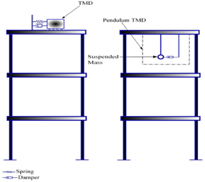 | Figure 3. MDOF system with a TMD at top |
Fig. 4 shows typical Fourier spectrum of the roof acceleration of the 5-DOF example building when the TMD is optimally tuned (i.e, {α, β} = 1). In order to see the effect of TMD, the Fourier spectrum are drawn up to frequency = 2 Hz. It can be seen that the resonant peak of the system without TMD is broken down into two peaks and shows two distinct closely spaced modes in the system with perfectly-tuned TMD. Moreover it can be observed that the Fourier amplitude is significantly reduced when the primary structure is installed with the TMD. Theoretically, when the TMD is perfectly tuned, the two resonant peaks attain the same amplitude in the spectrum. Fig. 5 shows the Fourier spectrum of the roof response for various values of α, α =0.8-1.2 with β =1.0. It can be seen that the absolute difference in the amplitudes of the resonant peaks increases with the de-tuning level.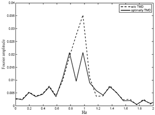 | Figure 4. Fourier spectra of the system with and without TMD |
3. Generation of Time-Series Model for a Class of Detuned Systems
It is quite obvious that the roof and TMD floor responses are most likely to be affected by the de-tuning level of TMD as compared to other floor responses. Hence an extensive time series analysis is performed with these responses. The idea is to simulate different class of time series models with reasonably wide range of (known or specified) detuning levels. Upon arrival of the experimental floor responses (with unknown de-tuning level of TMD), the corresponding time series model can be compared with the different class of models and then the unknown de-tuning level can be estimated.For example, in case of the 5-DOF building, the different class of model can be generated as shown in table 1 for various discrete values of α and β. In order to illustrate the method, typical time series analysis[11, 12] are described for Model-A63 (α=1 and β=1). α=1.0 and β=1.0 in the Model-A63 indicates the perfectly tuned condition. Extensive time series analysis of perfectly tuned (Model-A63) system using auto-regressive moving average (ARMA) model [11] is described next. In general, an ARMA (p,q) model for a zero mean time series can be written as: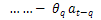 | (7) |
Using B operator, Eq. (7) can be written as: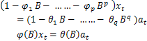 | (8) |
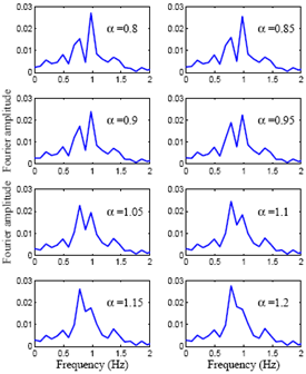 | Figure 5. Fourier spectrum of the roof acceleration for various level of de-tuning of stiffness with β=1.0 |
| Table 1. Various de-tuning levels in terms of α and β |
| | α|β | 0.0 | 0.5 | 1.0 | 1.5 | 2.0 | | 0.5 | A11 | A12 | A13 | A14 | A15 | | 0.6 | A21 | A22 | A23 | A24 | A25 | | 0.7 | A31 | A32 | A33 | A34 | A35 | | 0.8 | A41 | A42 | A43 | A44 | A45 | | 0.9 | A51 | A52 | A53 | A54 | A55 | | 1.0 | A61 | A62 | A63 | A64 | A65 |
|
|
3.1. Time Series Analysis for Model-A63
Time series of the roof and TMD floor accelerations are plotted in Fig. 6. It can be observed that the data has zero mean and approximately constant variance. Therefore the data can be treated as stationary time series. Fig.7 shows the Fourier spectra of the responses. The existence of five structural modes is observed in Fourier spectrum. Since the Model-A63 is optimally tuned, two resonant peaks of the roof response attain the same amplitude. However, the TMD floor primarily contains its own frequency and the first structural mode. Thus it can be fairly concluded that the number of required model order in the TMD floor response will be relatively low as compared to roof level response.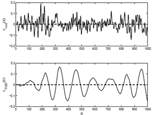 | Figure 6. Roof and TMD floor acceleration of the Model-A63 |
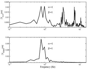 | Figure 7. Fourier spectra of the roof and TMD floor acceleration of the Model-A63 |
3.1.1. Identification
Fig. 8 and 9 shows the plots of sample auto-correlation function [11] (ACF) of the roof and TMD responses respectively with the 95% confidence limits (CL) above and below the axis. Four different CLs (depending on ρk =0 after a particular lag) are plotted in four different graphs. The estimated ACF has significantly non-zero values at lower lags and trends to follow a damped exponential curve. Because the theoretical ACF of an AR process behaves in this fashion, this indicates that perhaps some type of AR model would fit to these time series.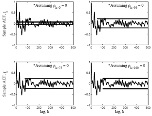 | Figure 8. Sample ACF of the roof response of Model-A63 |
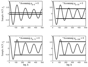 | Figure 9. Sample ACF of the TMD response of Model-A63 |
Fig. 10 shows the Sample partial ACF (PACF)[11] of the responses of the Model-A63.It can be observed that the PACF is attenuating in roof response and approximately cuts of at lag 9. Thus an AR(9) or an ARMA(9,q) model would be adequate. Whereas in case of TMD response, PACF cuts of at lower lag (say k =7). It strongly suggests to an AR(7) model. Fig. 11 shows the inverse ACF (IACF)[11] of the responses of the Model-A63. It can be observed that the IACF is attenuating in roof response and approximately cuts of at lag 6. Thus an AR(6) would be adequate. Whereas in case of TMD response, IACF cuts of at lower lag (say, k=1). It strongly suggests for an AR(1) model. Fig. 12 shows the inverse PACF (IPACF)[11] of the roof and TMD responses of the Model-A63. It can be observed that the IPACF is attenuating in both the responses. Thus it suggests that the AR type model is suitable for these time series. However the slow decay in the IPACF of TMD response indicates the existence of periodicity due to one/two frequency.Primarily it is identified that the AR(9) and AR(7) models are suitable for the roof and the TMD level responses respectively. Validation and adequacy of the identified model are checked through the confirmatory data analysis (estimation and diagnostic checks) respectively as described next. | Figure 10. Sample PACF of the roof and TMD response |
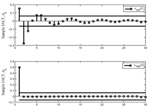 | Figure 11. IACF of the roof and TMD response of Model-A63 |
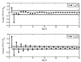 | Figure 12. IPACF of the roof and TMD response of Model-A63 |
3.1.2. Parameter Estimation
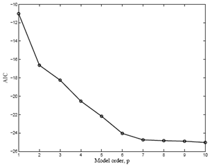
The method of maximum likelihood estimation (MLE) [16] is implemented to estimate the model parameters. To increase the speed, accuracy and simplicity the Akaike information criteria (AIC) [13] is commonly used. When there are several available models for modelling a time series, the model that posse minimum value of AIC should be selected. Fig. 13 shows the AIC values of the roof response for various model orders of an ARMA model. An ARMA(p,q) has been implemented and for a lower value of p, it can be observed that the AIC values are significantly low for higher q. However if p increases (for all q), AIC values are reducing further. But it is noted that the sensitivity of q is significantly low at higher value of p. Hence keeping in mind the model parsimony [11], an AR(9) model is selected for the roof response. This is the same model that was identified in the identification stage using PACF. Fig. 14 shows the AIC values of TMD responses for various model orders of AR model. Keeping in mind the model parsimony, an AR(7) model is selected for the TMD response.Once the model order is decided, some of the parameters of the best time series model are eliminated depending on their uncertainties. It can be achieved by using the standard error (SE) of MLE’s of the parameters [11]. Table 2 shows the details of the parameter estimation of the time series model of roof acceleration. The absolute values of the roots of φ(B) are greater than 1.0, thereby indicating the stationarity of the model. The estimation has been performed for the AR(9) model that has been identified in the identification phase and the same that satisfies the AIC criteria. It can be observed that the estimates of the parameters φ4 and φ7 are more than twice of their standard error. Hence the model AR(9) without φ4 and φ7 would be the proper model in terms of model parsimony. Table 3 shows the details of the parameter estimation of the time series model of TMD response. It can be observed that the estimates of the parameters φ2 to φ6 are more than twice of their standard error. Hence the model AR(7) without φ2 to φ6 is the proper model in terms of model parsimony.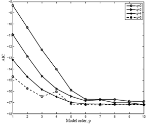 | Figure 13. AIC of the roof response w.r.t model order, p |
 | Figure 14. AIC of the TMD response w.r.t model order, p |
| Table 2. Parameter estimate and Validation of the Best model for Roof response |
| | φi | MLE | 2xSE | Abs. Roots of (B) | AIC | | φ1 | -2.07 | 0.06 | 1.36 | -24.75 | | φ2 | 1.03 | 0.14 | 1.36 | | φ3 | 0.41 | 0.15 | 1.32 | | φ4 | -0.07 | 0.159 | 1.32 | | φ5 | -0.27 | 0.159 | 1.11 | | φ6 | -0.18 | 0.159 | 1.11 | | φ7 | 0.07 | 0.158 | 1.14 | | φ8 | 0.28 | 0.14 | 1.18 | | φ9 | 0.158 | 0.0624 | 1.18 | | σa | 0.00498 | - | All roots > 1.0 |
|
|
Table 4 and 5 shows the details of the parameter estimation of the constrained model of the roof and TMD response. The estimation has been performed for the AR(9) model without the parameter φ4 and φ7 for roof response and the AR(7) model without the parameter φ2 to φ6 for TMD response. It can be observed that the estimates of all the parameters are less than twice of their standard error. Moreover, the AIC value of the constrained model is smaller than the previously obtained model.
3.1.3. Diagnostic Checks
Objective of these checks is to ensure that the chosen model adequately describes the time series under consideration by subjecting the calibrated model to a range of statistical tests. Primarily it checks the inherent assumption of the innovation series in terms of whiteness, normality and homoscedastic conditions [11]. As the first step, the innovation series  is estimated from the proposed model using following inverse expression of Eq. (8).
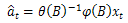 | (9) |
Whiteness can be checked through the residual autocorrelation function (RACF) [11] of  . Fig. 15 shows the plots of RACF calculated from roof and TMD responses and their corresponding proposed model as described in the last section. As shown in Fig. 15, except at very low lag, all RACF values are within the CL, therefore it can be concluded that the model is adequate.
| Table 3. Parameter estimate and Validation of the Best model for TMD response |
| | φi | MLE | 2xSE | Abs. Roots of (B) | AIC | | φ1 | -1.13 | 0.063 | 1.56 | -16.88 | | φ2 | 0.0056 | 0.0952 | 1.54 | | φ3 | 0.0057 | 0.0952 | 1.54 | | φ4 | 0.0051 | 0.0952 | 1.43 | | φ5 | 0.004 | 0.0951 | 1.43 | | φ6 | 0.003 | 0.095 | 1.03 | | φ7 | 0.122 | 0.0628 | 1.03 | | σa | 0.00537 | - | All roots > 1.0 |
|
|
| Table 4. Parameter estimate and Validation of the Constrained model for Roof response |
| | φi | MLE | 2xSE | AIC | | φ1 | -2.2 | 0.06 | -29.6 | | φ2 | 1.13 | 0.14 | | φ3 | 0.43 | 0.15 | | φ5 | -0.32 | 0.11 | | φ6 | -0.28 | 0.17 | | φ8 | 0.35 | 0.11 | | φ9 | 0.15 | 0.07 | | σa | 0.005 | - |
|
|
| Table 5. Parameter estimate and Validation of the Constrained model for TMD response |
| | φi | MLE | 2xSE | AIC | | φ1 | -1.9 | 0.078 | -17.2 | | φ7 | 0.15 | 0.072 | | σa | 0.0054 | - |
|
|
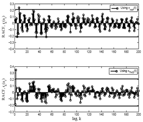 | Figure 15. RACF at various lags |
In order to check the normality of the innovation series, the skewness (g1) and the kurtosis coefficients (g2) are computed and compared against the hypothesis testing. The g1 values of t computed from the roof and TMD responses are -0.018 and -0.057 respectively. Thus it satisfies the normality condition (as g1=0.0 for a normal data). The g2 values of the  computed from the roof and TMD responses are -0.057 and -0.02 respectively. Thus it satisfies the normality condition (as g2 =0.0 for a normal data). Hence both the
  series as estimated from the roof and TMD responses satisfies the normality condition. Alternatively, normal probability paper plot can also be used to identify normality in the
  series. Fig. 16 shows the normal probability paper plot for the
  series as estimated from the roof and TMD responses. Linear pattern of the scattered data confirms the normality of the
  series.
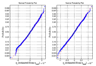 | Figure 16. Normal probability paper plot for at series of Model-A63 |
4. Simulation
One of the important uses of time series model is simulation. The goal of the simulation is to employ the fitted model to generate any possible set of stochastically equivalent sequences of observations which could occur in future. Well-known simulation procedure, Waterloo simulation procedure 3 [11] is used for this purpose. Fig 17 shows the simulated (synthetic) time series of (best constrained) Model-63 as obtained in table 4 and 5 using unit residual variance. It is observed that the dynamical properties of these synthetic time series are quite similar to the respective original time series as shown in the beginning of this section. This indicates the efficacy of the simulation procedure.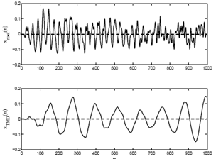 | Figure 17. Simulated time series of Model-A63 |
5. Validation
In order to validate the proposed time series technique, 6 time series models (A11, A21, A31, A41, A51 and A61) are considered as described in Table 1. The simulations are performed to generate roof accelerations using the fitted time series models as described in the previous sections. In the absence of any experimental data, it is assumed that the model A41 is the model whose de-tuning level is un-known and its actual response is available. Therefore the actual (not simulated) response of Model−A41 (defined as Model−U with unknown detuning level) serves as an experimental data. The basis of the present study is to show how the time series models can be used to detect the unknown de-tuning level of TMD. Hence in summary, the proposed time series technique is implemented to estimate the unknown de-tuning level of ”actual” A41 model or Model−U using a class of 6 synthetic models.A performance index in terms of root-mean-square (RMS) error is used to compare the true and simulated time series. Fig. 18 shows the RMS error of the response and simulated responses from six synthetic models. It can be observed that the RMS error attains minimum value corresponding to the Model−A41, Hence it can be concluded that the level of de-tuning level of Model−U is same as in the simulated model of A41. Thus the de-tuning level (α = 0.8 and β = 0.0) is detected correctly.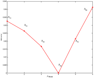 | Figure 18. RMS error in different class of synthetic models |
6. Conclusions
In the present study, a time-series analysis based technique for identifying the de-tuned level of any TMD-installed structural system is proposed. A class of several de-tuned models are simulated based on the finite element model of the system and the corresponding time series models are formed. Upon arrival of the experimental or real-life data, they can be compared with the set of different class of time series model and the unknown de-tuning level of the real life structure can be estimated. The method, however, require an up-to-date finite element model of the real-life structure. The present study describes the validity and usefulness of the time series model in a detail manner and an idea of estimation of unknown de-tuning level are proposed. As a future work, the current technique will be implemented in the ambient vibration response of a real-life TMD-installed building.
References
| [1] | Spencer,B.F. and Nagarajaiah,S., 2003, State of the art of structural control, J. of Struc. Eng.,ASCE, 129(7), 845-856 |
| [2] | A. Kareem, and T.Kijewski, 1999, Mitigation of motions of tall buildings with specific examples of recent applications, Wind and Structures, 2(3), 201-251 |
| [3] | K. C. S. Kwok and B. Samali, 1995, Performance of tuned mass dampers under wind loads, Engineering Structures, 17(9), 655-667 |
| [4] | Lari Kela and Pekka Vahaoja, 2009, Recent studies of adaptive tuned vibration absorbers/neutralizers, Applied Mechanics Reviews, 62(6) |
| [5] | M. Abe and Y. Fujino, 1994, Dynamic characterization of multiple tuned mass dampers and some design formulas, Earthquake Engineering and Structural Dynamics, 23, 813-835 |
| [6] | DenHartog, J.P., Mechanical Vibration (New York:McGraw-Hill, 1956) |
| [7] | Warburton, G.W., 1982, Optimum absorber parameters for various combinations of response and excitation parameters, Earthquake Engineering and Structural Dynamics, 10(3), 381-401 |
| [8] | Rana,R., and Soong, T.T., 1998, Parametric study and simplified design of tuned mass dampers, Engineering Structures, 20(3), 193-204 |
| [9] | Gerges, R.R., and Vickery, B.J., 2005, Optimum design of pendulum-type tuned mass dampers, The Structural Design Of Tall and Special Buildings, 14(4), 353-368 |
| [10] | Hazra, B., and Sadhu, A., and Lourenco, R., and Narasimhan, S., 2010, Retuning tuned mass dampers using ambient vibration response, Smart Materials and Structures, 19(2), 13pp |
| [11] | Hipel, K. W., and Mcleod, A. I., Time Series Modelling of Water Resources and Environmental Systems (Amsterdam, Netherlands: Elsevier, 1994) |
| [12] | Box, G. E. I, and Jenkins, G. M., and Reinsel, G. C., Time Series Analysis: Forecasting and Control (Hobo-ken,New Jersey: JohnWiely and Sons, 2008) |
| [13] | Akaike, H.,A new look at the statistical model identification, 1974, IEEE Transactions on Automatic Control, 19, 716-723 |
| [14] | B. Hazra, A. Sadhu, A. J. Roffel, S. Narasimhan, 2011, Hybrid Time-Frequency Blind Source Separation Towards Ambient System Identification of Structures, Computer-aided Civil and Infrastructure Engineering,DOI: 10.1111/j.1467-8667.2011.00732.x, 12pp |
| [15] | Maia et al, 1997, Theoretical and experimental modal analysis, Research studies press, Taunton, Somerset, UK |
| [16] | L. Ljung, 1999, System Identification: Theory for the user, Prentice Hall, Inc, Upper Saddle River, New Jersey 07458 |
 Abstract
 Reference
 Full-Text PDF
 Full-Text HTML