-
Paper Information
- Next Paper
- Paper Submission
-
Journal Information
- About This Journal
- Editorial Board
- Current Issue
- Archive
- Author Guidelines
- Contact Us
Journal of Mechanical Engineering and Automation
p-ISSN: 2163-2405 e-ISSN: 2163-2413
2011; 1(1): 1-7
doi: 10.5923/j.jmea.20110101.01
Numerical Model to Study of Contact Force in A Cylindrical Roller Bearing with Technical Mechanical Event Simulation
 Abstract
 Reference
 Full-Text PDF
 Full-Text HTML
Laniado-Jacome Edwin
Mechanical engineering department, Carlos III University, Madrid, 28911, Spain
Correspondence to: Laniado-Jacome Edwin , Mechanical engineering department, Carlos III University, Madrid, 28911, Spain.
| Email: |  |
Copyright © 2012 Scientific & Academic Publishing. All Rights Reserved.
A study of contact force between rollers and races in a roller bearing with a numerical model for mechanical event simulations bearing is presented in this paper with different load type on shaft. These numerical models provide with the spatial and time distributions of stress and strain values, as well as all the nodal displacements at every time step. The model was developed with the finite element method (FEM) for mechanical event simulations (MES) with the commercial code AlgorTM. The model has been validated by verifying that the contact force distributions correspond to those predicted by the analytical model of Harris-Jones.
Keywords: Mechanical Event Simulation, Finite Element Method, Roller Bearing
Cite this paper: Laniado-Jacome Edwin , "Numerical Model to Study of Contact Force in A Cylindrical Roller Bearing with Technical Mechanical Event Simulation", Journal of Mechanical Engineering and Automation, Vol. 1 No. 1, 2011, pp. 1-7. doi: 10.5923/j.jmea.20110101.01.
Article Outline
1. Introduction
- There are some studies of the dynamic behavior of bearings, which have very advanced methods of analysis of vibration frequency, but it is difficult to obtain data to generate magnitudes of stress and deformation of the rollers on the races[1-4]. The analysis of experimental models bearing, the method is not sufficient to isolate the signal of movement due to deformation of the load with other signals that are mixed and are known as noise because of this, this work proposes bearing valid model for results of contact[12,13]. This paper proposes a numerical model of cylindrical roller bearing at different speeds of planar rotation in the shaft (30, 40, 50 and 100Hz) with three degrees of freedom in each node to analyze the contact between rollers with outer race. This is due mainly to the huge computation resources required when many surfaces are to be in contact during a dynamic simulation. Although it varies from one software to another, we can say that the contact between two surfaces A and B, having NA and NB nodes respectively, involves one contact element for every pair of nodes, which adds up to NA•NB contact elements. To give an example, a 3D numerical model of a 10-ball bearing, with 500 nodes on each ball surface and 500 on each race (inner and outer) surface, requires 5 million contact elements. Note that the velocities concerning rolling bearings demand high time resolution, which leads to extremely large simulations, hav-ing many time steps.To summarize, mechanical event simulations of dynamic phenomena in rolling bearings, like sliding, are, to a certain extent, unapproachable with 3D numerical models and ex- perimental models[2,5,6,7]. In this paper, a 2D numerical model has been modeled with three degrees of freedom per node for mechanical event simulations of a roller bearing is firstly presented on an analysis of the mechanical behaviour and as data for important contact between the rollers and the outer race. With this model, many simulations have been carried out under the finite element commercial software Algor™[8] for different shaft rotation velocities with a radial load applied at its centre. The software provides stress, strains and displacements at each point, for each time step, as well as the contact force on every node involved in the contact between the rolling elements and the races. The numerical model presented is validated by comparing the load distribution over the outer ring it provides with that according to the counterpart analytical model of Jones- Harris. The formulation of this analytical model and the results it provides concerning the contact force distribution particularized for a rolling bearing identical to the FE/MES modeled. The analysis for the two models for each shaft speed is performed with relative difference on the outer race on the load zone. The steps followed for this research are as follows.Numerical model presented is a cylindrical roller bearing with boundary conditions similar to a model of experimental bearing.Discusses the results of numerical model to find the boundaries of contact within the cargo area for each speed of rotation.This article shows an analytical model of Harris-Jones [9,10] applying the same external and internal conditions have numerical model.The Harris-Jones model of a roller bearing provides a system of non-linear equations that is resolved with the data analysis program MathCad™[11].An analysis of the relative error between the two models, the numerical model simulated dynamically by means of finite element method in mechanical event simulation and analytic model Harris-Jones.That is why some authors have performed analytical models with mathematical formulation for analyzing the results of the contact forces on the races[14,15], but the results of these models do not analyze dynamic phenomena such as deformed during early bearing operation, the sliding between mating parts, fatigue, among others.The way to obtain the contact force distribution from numerical model simulations with the proposed model is shown. Then the corresponding data are compared to those presented, which results in the validation of the proposed model.
2. Numerical Model of the Cylindrical Roller Bearing
- There are different types of bearing; among the most used in industry are the bearings with balls and cylindrical roller bearings for high load[16]; for this study used the roller cylindrical bearing to study the dynamic behavior and surface contact rollers and races, the main components of this bearing (except for the cage, seals, and other non-loaded components) are basically cylinders whose axes are parallel to each other and to the bearing axis. The dynamics of the system moves on a plane, on the plane normal and the forces between components, as well as the external one, also lie in planes that are parallel to the movement plane: it is a plane stress problem.The model of the bearing has a shaft with the inner ring, 13 rolling elements (rollers), the outer ring, the cage, and a system of radial elements that gives the prescribed speed to the shaft; adds a new piece is called "motor torque" is applied to control the speed of rotation of the shaft.
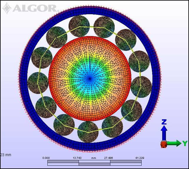 | Figure 1. 2D numerical model of the a roller cylindrical bearing |
|
3. Analytical Model
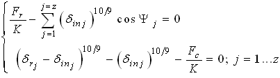
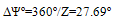
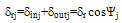
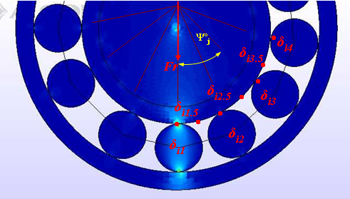
- The analytical model proposed for a bearing in this research is the Harris-Jones model for a cylindrical roller bearing, this model is generated from the Hertz contact formulation and dynamic balance[17,18]. This model provides a system of non-linear equations composed of one equation for the force balance of the shaft (which is under a radial force applied at its centre), and one more for each of the loaded rollers (j=1…z), which undergo the contact forces from the inner and outer races as well as the centrifugal force of inertia:Figure 2 shows the point where the radial force (Fr) is applied and the contact forces in response to applied force on the center shaft. Contact forces are calculated initially on the contact points of the rollers on the inner race.
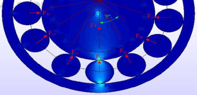 | Figure 2. Radial force applied and contact forces on the bearing |
 | (1) |
 | (2) |
 | (3) |
 | (4) |
 | (5) |
|
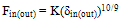
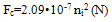
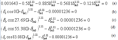 To solve this nonlinear equation system using the MathCad™ program, entering the solution of the linearized system as the seed for the non-linear one. The error (absolute zero) of this method was less than 10-5. Finally, the values of the contact forces the outer race exerts on each of the loaded rollers can then be easily obtained from Eq. N:
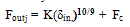 | (6) |
|
 | Figure 3. Deformation points on the inner race |
 | Figure 4. Load zone on outer race to 100 Hz |
4. Numerical Model Contact Force Data
- Data acquisition of the numerical model took into account several factors that met the following dynamic conditions.Rotation speed of constant shaft.There is of rolling effect between the rollers and racesExistence of nodes of contact between rollers and races (table 2) Distance between nodes relatively small to avoid small rebounds.The mesh of the roller and the inner and outer rings with the contact nodes that are generated are the critical elements involved in the formation of bearing numerical model, which is why you should follow these conditions:
|
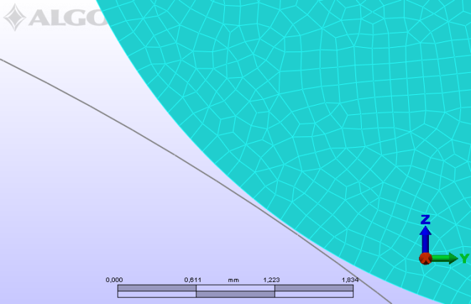 | Figure 5. Conditions of meshing for roller |
 | Figure 6. Nodes involved in the contact |
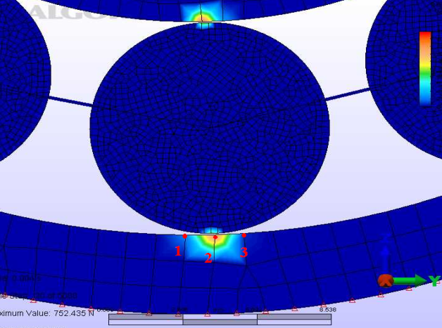
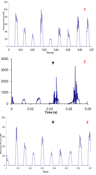 | Figure 7. Scheme for the reaction force in the numerical model |
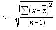 | (7) |
|
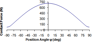
 | Figure 8. Reaction force with deviation on load zone |
5. Validation with Relative Difference between Models
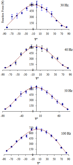
- Is validated by comparison of two theoretical models, is not defined experimental model because of the difficulty of acquiring data of contact between the rolling elements and the rings of a bearing. The analytical model shown in this study of the dynamic equilibrium equations of Harris and Jones proposed to determine the reaction force within the load zone for this study assumes that forces the load zone are low magnitude.The validation of the numerical model of a cylindrical roller bearing for this research was conducted by comparison with the analytical model of Harris - Jones with similar features and equal boundary conditions. The validation was performed by comparing the reaction force exerted by way of the rollers on the outer race in the load zone for both models.For a real validation have been described the geometry of the load zone for each model, the description of the load zone will serve to better demonstrate the dynamic behavior of the numerical model compared with the analytical model.
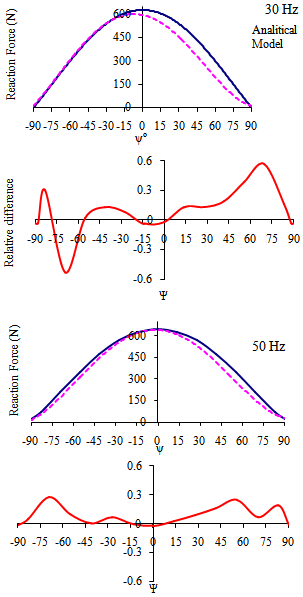 | Figure 9. Load zones of analytical and numerical 30, 40, 50 and 100 Hz models |
6. Conclusions
- Conditions and characteristics applied to the numerical model of a cylindrical roller bearing are similar to the experimental design, but although the signals and data acquired from the analysis of numerical model are as close to a real model known.Numerical model of a cylindrical roller bearing has been validated through the optimum analytical model proposed by Harris-Jones without major differences. Presented differences are because the dynamic numerical model presents phenomena that are manifest in the load zone is not symmetrical.The numerical model presented phenomena of an experimental model; these phenomena are due to the dynamics of the system, where you can explore different events as chaotic behavior of the rolling elements, falls, blows, slipping between the races and rollers, among others.Numerical model generates the geometry of the load zones adapted to the dynamics of the bearing elements in contact with geometry it may predict behavior, failure, location of critical areas among others.
References
| [1] | S. Braun, "Mechanical signature analysis of sonic bearing vibrations," IEEE Transactional on Sonic and Ultrasonics, vol. 27, pp. 317-328, 1980 |
| [2] | Z. Kiral and H. Karagülle, "Vibration analysis of rolling element bearings with various defects under the action of anunbalanced force," Mechanical Systems and Signal Processing, 2005 |
| [3] | R. Rubini and U. Meneghetti, "Application of the Envelope and Wavelet Transform Analyses for the Diagnosis of Incipient Faults in Ball Bearings," Mechanical Systems and Signal Processing, vol. 15, pp. 287-302, 2001 |
| [4] | S. Wang, W. Huang and Z. K. Zhu, "Transient modeling and parameter identification based on wavelet and correlation filtering for rotating machine fault diagnosis," Mechanical Systems and Signal Processing, vol. 25, pp. 1299-1320, 2011 |
| [5] | Zienkiewicz, O.C. and Cheung, Y.K., The Finite Element Method in Structural and Continuum Mechanics. New York: MacGraw-Hill, 1967 |
| [6] | Sawalhi, N. and Randall, R.B., "Simulating gear and bearing interactions in the presence of faults Part I. The combined gear bearing dynamic model and teh simulation of localised bearing faults," Tribology International, vol. 22, pp. 1924-1951, 2008 |
| [7] | I. A. Zverev, I. -. Eun, W. J. Chung and C. M. Lee, "Simulation of Spindle Units Running on Rolling Bearings," International Journal of Advanced Manufacturing Technology, vol. 21, pp. 889-895, 2003 |
| [8] | ALGOR™. (2008, License number DE23692. I+D+I. professional multiphysics. MES. 19 |
| [9] | T. A. Harris, Rolling Bearing Analysis. New York, U.S.A.: 1991 |
| [10] | A. Jones, "A general theory for elastically constrained ball and Roller bearing under arbitrary load and Speedy conditions." vol. 105, pp. 591-595, 1960 |
| [11] | MATHCAD™., "License Universidad Carlos III de Madrid. PTC," vol. 14, 2005 |
| [12] | S. Braun, Discover Signal Processing. An Interactive Guide for Engineer. 2008 |
| [13] | B. K. Bae and K. J. Kim, "A Hilbert transform approach in source identification via multiple-input, single-output modelling for correlated inputs," Mechanical Systems and Signal Processing, vol. 12, pp. 501-513, 1998 |
| [14] | S. Harsha, "Nonlinear dynamic analysis of an unbalanced rotor supported by roller bearing. Chaos, Solitons and Fractal," Chaos, Solitons and Fractal, vol. 26, pp. 47-66, 2005 |
| [15] | N. Tandon and A. Choundhury, "An analytical model for the prediction of the vibration response of rolling element bearings due to localized defect," Journal of Sound and Vibration (1997) 205 83), 275-292., pp. 275-292, 1997 |
| [16] | S. Orhan, N. Aktürk and V. Celik, "Vibration monitoring for defect diagnosis of rolling element bearings as a predictive maintenance tool," Comprehensive Case Studies NDT&E International, vol. 39, pp. 293-298, 2006 |
| [17] | H. Hertz, "Über die Berührung fester elastischer Körper " J. Reine Angew Math, vol. 92, pp. 156-71., 1882 |
| [18] | Kang, Y., Shen, P., Huang, C., "A modification of the Jones-Harris method for deep-groove ball bearings," vol. 39, pp. 1413-1420, 2006 |
| [19] | P. J. L. Fernandes, "Contact fatigue in rolling-element bearings," Engineering Failure Analysis, vol. 4, pp. 155-160, 1997 |