-
Paper Information
- Paper Submission
-
Journal Information
- About This Journal
- Editorial Board
- Current Issue
- Archive
- Author Guidelines
- Contact Us
Journal of Laboratory Chemical Education
p-ISSN: 2331-7450 e-ISSN: 2331-7469
2022; 10(2): 25-37
doi:10.5923/j.jlce.20221002.02
Received: Jul. 4, 2022; Accepted: Aug. 3, 2022; Published: Aug. 15, 2022

Microsoft Excel Solver-assisted Composition Determination to Improve the Experiment of Liquid-Vapor Phase Diagram Construction
 Abstract
 Reference
 Full-Text PDF
 Full-text HTML
Hong Shen, Yayue Mei, Tingxue Xie
Institute of Analytical Chemistry, Department of Chemistry, Zhejiang University, Hangzhou, China
Correspondence to: Hong Shen, Institute of Analytical Chemistry, Department of Chemistry, Zhejiang University, Hangzhou, China.
| Email: |  |
Copyright © 2022 The Author(s). Published by Scientific & Academic Publishing.
This work is licensed under the Creative Commons Attribution International License (CC BY).
http://creativecommons.org/licenses/by/4.0/

Since liquid-vapor equilibrium is one of the essentials in thermodynamics to design and optimize separation processes, and phase equilibria require a good understanding of phase diagrams, “Constructing Liquid-Vapor Phase Diagram for Two Completely Miscible Components Systems” often serves as a common experiment in physical chemistry course. In the experiment, the compositions of the binary system, determined both from the liquid and the vapor phases at equilibrium, are regarded as the key data in deriving the overall system point in phase diagram. Here, a practical computer-assisted data processing protocol by using Microsoft Excel Solver is introduced for obtaining the system composition. Combined with the measured refractive index of a standard mixture of the binary system, the composition of any sample mixture of the system can be optimally solved from its refractive index for the phase diagram construction. The paper presents the attempt to improve the experiment, displaying the optimally-solving procedure. The accuracy and feasibility of the approach are verified, and its expanding application prospect in differential refractive index detection are discussed.
Keywords: Phase Diagram, Excel Solver, Composition Determination, Refractive Index
Cite this paper: Hong Shen, Yayue Mei, Tingxue Xie, Microsoft Excel Solver-assisted Composition Determination to Improve the Experiment of Liquid-Vapor Phase Diagram Construction, Journal of Laboratory Chemical Education, Vol. 10 No. 2, 2022, pp. 25-37. doi: 10.5923/j.jlce.20221002.02.
Article Outline
1. Introduction
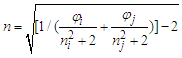
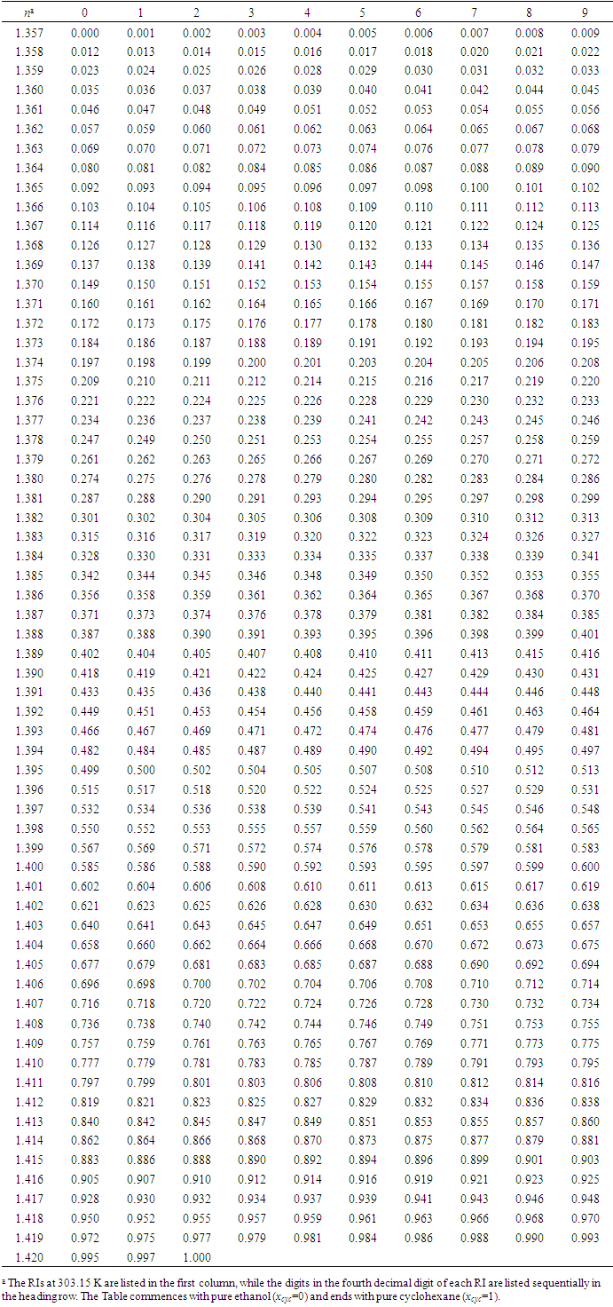
- Phase equilibria have great significance in chemical engineering and chemical process technology. Liquid-vapor equilibrium is one of the most common phase equilibria in practical applications, such as in chemical, petrochemical, pharmaceutical and food industries. Liquid-vapor equilibrium data, graphically presented in phase diagrams, are the basis of developing distillation (or rectification) technique for separating liquid mixtures into pure substances. As a common experiment in physical chemistry laboratory, “Constructing Liquid-Vapor Phase Diagram for Two Completely Miscible Components Systems” helps students learn to determine the liquid-vapor equilibrium (i.e., boiling point) parameters, so as to enhance both the comprehension of solution thermodynamics theory and the skills of experimental operation. In view of the phase equilibrium data being the basis of phase separation, the composition determination of the binary mixture is believed to be one of the key steps in the experimental practice [1-5].Determining the composition or components amount of the binary mixture at phase equilibrium is generally based on the refractive index (RI) measurement or via using chromatography analysis, of which, the former is widely used due to its simplicity in operation and low capital investment [1-2]. The method used to measure the refractive indices (RIs) of a series of binary standard solutions at a certain temperature, and establish a “Correlation Table of RIs against Compositions” (e.g., RIs vs. mole fraction x, as refer to Table S1 in the Supplementary Material (1) used in Zhejiang University); thus, the composition of the binary sample solution, either in the liquid or vapor phase, can be determined depending on its measured RI value (the RI of vapor obtained from its condensate solution). However, limited by various factors such as analytical instrument accuracy, measurement temperature and sample size, etc., it is impossible to experimentally collect all arbitrary data into the correlation table, so those unmeasured data often need to be supplemented through interpolation. If simple piecewise linear interpolation is used, the RI of binary mixture should preferably be one that varies apparently and smoothly over its entire composition range. If more complex interpolation model, such as Newton or Lagrange interpolation is employed, typically relevant mathematical and software skills are required, which hardly matches majority of undergraduate students. In practice, however, once the RI of a sample solution is measured, the student experimenters always just look up the correlation table to find its composition without the comprehension of where the data in the table come from or how the interpolations are carried out, and thus they are not really involved in all of the phase equilibrium data acquisition and processing.RI measurement is one of the essentials for determination of composition of binary mixtures, usually for non-ideal mixtures where direct experimental measurements are performed over the entire composition range. The widely used rules for predictivity of refractivity in case of binary liquid mixtures are Arago-Biot, Gladstone-Dale, Lorentz-Lorenz, Eykman, Weiner, Heller, Newton, Oster and Eyring-John [6]. Among them, the most reliable empirical equation over a wide range of concentration is the Lorentz-Lorenz equation (i.e., L-L equation) [7-10] as follows,
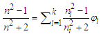 | (1) |
 | (2) |
 | (3) |
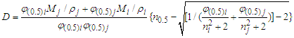 | (4) |
2. Optimally-Solving Procedure
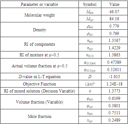
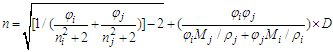
- Simulation of various mathematical models via Excel Solver to obtain the optimal solution (i.e., the “Variable” to be solved) can be accepted as a simple and practical means by setting the “Decision Variable” of the “Objective Function” under various conditions (such as maximum, minimum and specified). Especially, when the “Objective Function” is specified as zero, it becomes solving an equation. But to avoid computational overfitting, such “Objective Function specified as zero” is usually replaced by “square of the Objective Function specified as minimum”. Sometimes, certain additional constraints are attached as well to discard the unreasonable solved results.For this work of inversely solving the L-T equation to find the composition with known RI of the sample mixture, taking measured RI (n) as the “Decision Variable”, the difference between the solved RI (nsolved) and the measured RI (n) as the “Objective Function” to be minimized (i.e., (Δn)2≈0), then with some additional “Constraints” to derive a reasonable result, the “Variable” to be optimally solved (i.e., the composition φi) can be obtained via Excel Solver programming. Specifically, taking ethanol−cyclohexane mixture as an example, the optimally-solving procedure is described as follows and shown in Figure 1 (also with an Excel template file attached as the Supplementary Material (2)).1. An Excel spreadsheet is established with all relevant data included. 2. Click the Solver icon on the “Data Toolbar” to start the Solver, the “Solver Parameter” window is opened up wherein the blanks of “Set Objective” and “By Changing Variable Cells” are needed to be filled with specific cell info to define the “Objective Function” and the “Variable (Decision Variable to be solved)”. Then, set some additional “Constraints” in the blank of “Subject to the Constraints”, because the composition should be limited in the range of 0 to 1. 3. Calculate the D-value of the L-T equation according to Eq. 4 with a series of relevant parameters of a standard ethanol−cyclohexane mixture and its components (e.g., n(0.5), φ(0.5)eth, φ(0.5)cyc, Meth, Mcyc, ρeth, ρcyc, neth, ncyc, specifically with the known φ(0.5)eth or φ(0.5)cyc near 0.5). 4. Set the “Objective Function” (Δn)2 to be minimized.5. Preassign an arbitrary initial value of composition (e.g., φeth=0.5) and execute Solver process to obtain the solved composition of the ethanol−cyclohexane sample mixture (i.e., φeth, φcuc, xeth, xcyc) based on the measured RI (n) of sample mixture, the calculated D-value and the components parameters (e.g., Meth, Mcyc, ρeth, ρcyc, neth, ncyc). Noted for the “Select a Solving Method” option, choose “Nonlinear GRG” (suitable for the nonlinear “Objective Function” of this work).
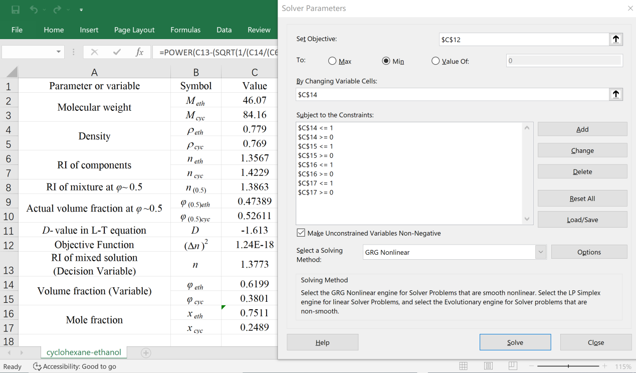 | Figure 1. Excel spreadsheet with Solver dialog window for solving the composition of ethanol−cyclohexane mixture (assumed as ideal solution in φ and x conversion 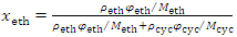 |
3. Results and Discussion
3.1. Comparative Features of the Composition Determination
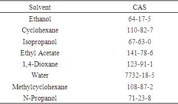
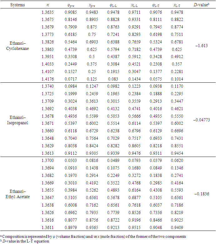
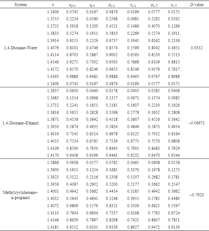
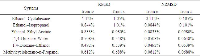
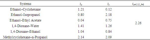
- To verify the feasibility of the proposed approach, seven binary systems with various components that were hopefully suitable for student experiments were prepared. All reagents used were of analytical grade (see CAS numbers in Table S2 in the Supplementary Material (1)) and the RIs were obtained at 298.15 K with an Abbe refractometer (Shanghai INESA Scientific Instrument Co., Ltd., China) carried out at the standard wavelength of 589.3 nm (nD) as the light source. The optimally-solved compositions obtained via Excel Slover programming, either based on the L-T or the L-L equation (taking the latter as the control), were compared with the actually-prepared compositions (see Table S3, S4 in Supplementary Material (1) for data) as depicted in Figure 2 and Figure 3.
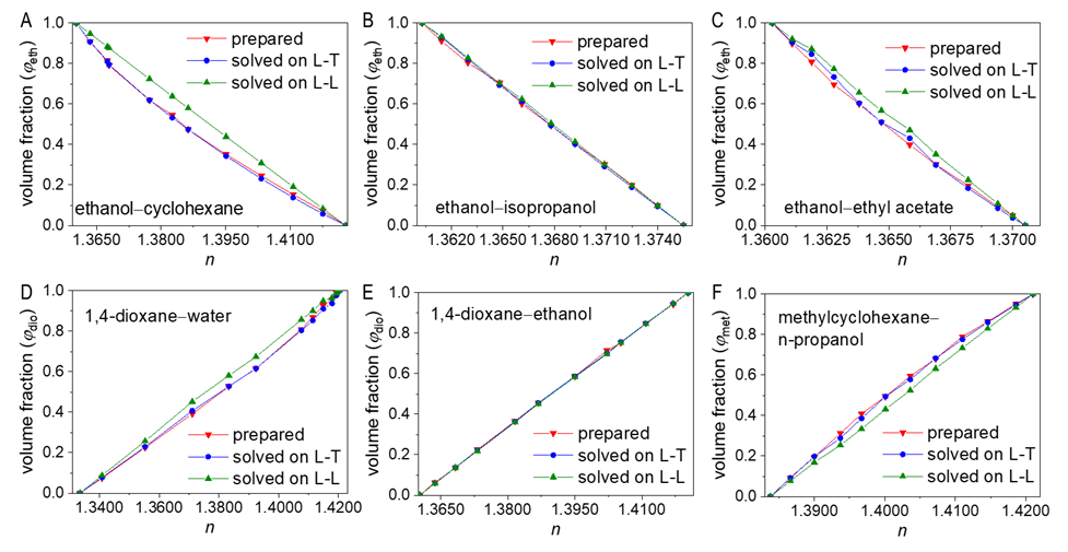 | Figure 2. Comparison of the actually-prepared compositions of six binary mixtures with those optimally-solved based on the L-T or the L-L equation |
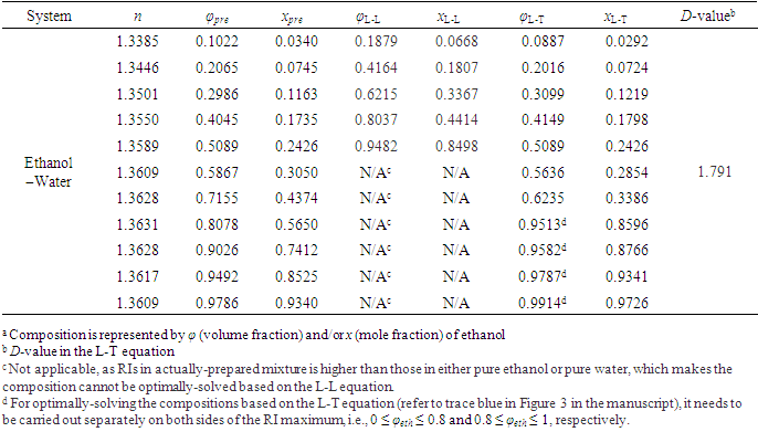
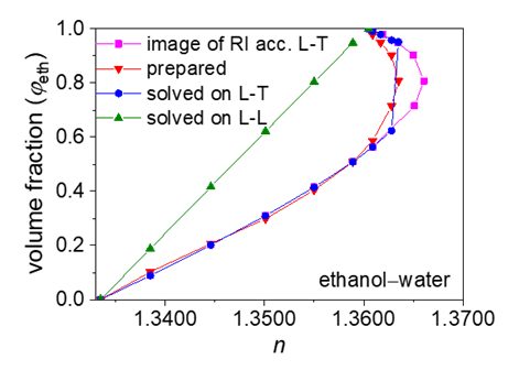 | Figure 3. Comparison of the actually-prepared compositions of ethanol-water mixture with those optimally-solved based on the L-T or the L-L equation, and those from the image of the RI function according to the L-T equation (Note: for optimally-solving on the L-T equation to obtain trace blue, it needs to be carried out separately on both sides of the RI maximum, i.e., 0 ≤ φeth ≤ 0.8 and 0.8 ≤ φeth ≤ 1, respectively.) |
3.2. Phase Diagram Construction Practice
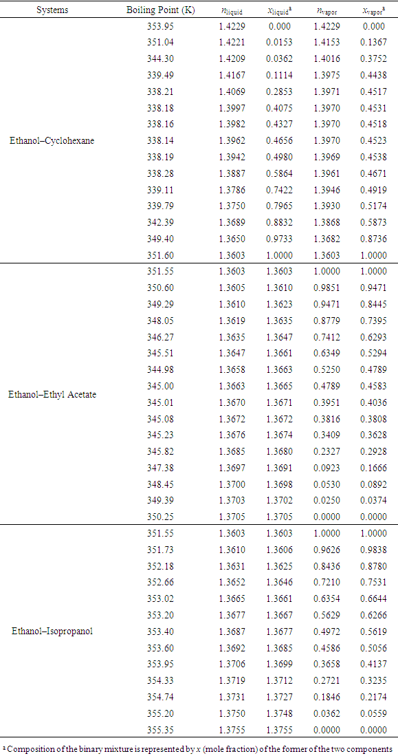
- According to previous practice, the experiment “Constructing Liquid-Vapor Phase Diagram for Two Completely Miscible Components Systems” generally relies on the “Correlation Table of RIs against Compositions” of the system. The more accurate the experiment is expected, the more standard solutions need to be prepared. However, to save the class time, such correlation table is actually provided in advance, which might give students a misconception that the experiment should be performed on binary system with known RI/composition correlation, so they cannot generalize the experiment from one system to the other. The proposed approach, by using Excel Solver to solve the composition, brings two changes. First, instead of preparing a series of standards to establish the RI/composition correlation table, it requires just one standard solution. Then, the composition of the binary mixture at phase equilibrium, either in liquid or in vapor phase, can be easily solved via entering the RI of the solution (or condensate solution) into Excel spreadsheet. Here, as shown in Figure 4, the phase diagrams of three binary systems have been constructed, including ethanol−cyclohexane, ethanol−ethyl acetate, and ethanol−isopropanol, selected for their mild operation temperature, green and less corrosive solvents for safe experimentation. The phase diagrams constructed from the compositions solved on the L-T equation via Excel Solver (see Table S7 in Supplementary Material (1) for data) are in good consistent with those reported previously [20-22], demonstrating the feasibility of the proposed approach for student’s experiment.
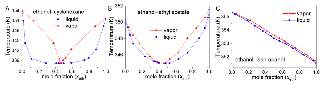 | Figure 4. Phase diagrams constructed from the optimally-solved compositions based on the L-T equation |
4. Expanding Application Prospect
- In fact, determination of analyte concentration in a mixed sample solution from its measured RI is also a common type of quantitative analysis, such as during HPLC separation. Differential refractive index (DRI) detector offers attractive characteristics as non-destructive and universal sensor, estimating analyte concentration (φa) by monitoring the difference of RIs (nDif) between the sample (nS, the RI of analyte−eluent mixed solution) and the reference (nR, the RI of blank eluent) [23]. In previous studies based on DRI detection, two quantitative formulas have been proposed successively from the perspective that the detected signal (nDif) shows linearity in a certain analyte concentration range.Yeung et al. [24,25], by derivation of the L-L equation, proposed a protocol for determining the volume fraction of analyte (φa) in a flowing system, involving a variety of binary systems with the solvents, such as n-hexane, benzene, chloroform, carbon tetrachloride and carbon disulfide. The quantification equation is as follows,
 | (5) |
 is a constant term related to the RI of the blank eluent (nR);
  and
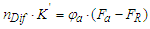
and  are equivalent to the molar refractivities per unit molar volume (Rm/Vm) of the analyte and the blank eluent, respectively. Obviously, the formula shows the nDif is proportional to the φa of the sample solution, as well as to the difference of molar refractivities between the analyte and the eluent that affects the linear slope. Actually, this formula results from the substitution of nR for nS during its derivation [24], suggesting it can just be applicable to the system with low analyte concentration (φa ≤ 5%) [26].Then, Dorschel et al., the scientists from the Waters Chromatography Division, modified the above formula (Eq. 5) according to their practice of DRI detector to obtain a revised equation [26],
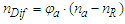 | (6) |
5. Conclusions
- As students develop their cognitive learning abilities and scientific process skills, computational formulas, content, and procedures have become increasingly integrated. The data processing in chemical experiment course, often due to its complexity or cumbersomeness, calls for computer-assisted calculation to replace some repetitive experimental operations or manual calculation, becoming one of the important requirements. Here, we show how to use spreadsheet modeling of Microsoft Excel Solver to solve a nonlinear optimization problem, making it easy to determine the composition of a completely miscible binary system. The paper proposes a protocol to improve the experiment “Constructing Liquid-Vapor Phase Diagram for Two Completely Miscible Components Systems”, reducing errors caused by individual operational differences. The approach helps students to better understand the principle of phase diagram construction with improved data processing capability, and also shows its expanding application prospect worthy of study further.
Supplementary Material (1)
|
|
|
|
|
|
|
|
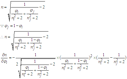 With
With 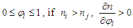 . And in the opposite, if
  .Proof 2. Proof of either monotonic or non-monotonic function of compositions (φ) according to the L-T equation.
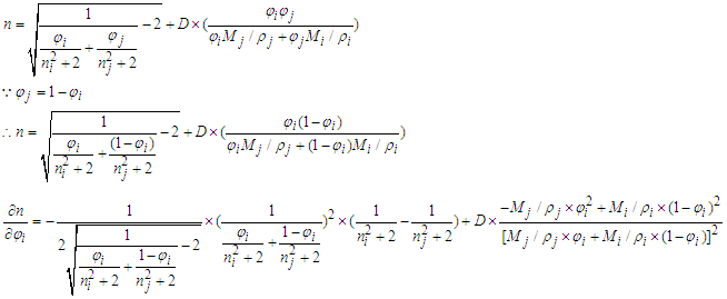 (1) For ethanol–cyclohexane system, component i is ethanol.
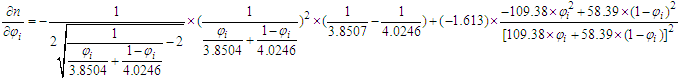 With
With  and the RI of the mixture decreases with the increase of mole fraction of ethanol.(Refer to Table S3 for D value)(2) For ethanol–water system, component i is ethanol.
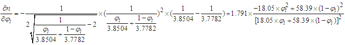 If
If  and the RI of the mixture increases with the increase of mole fraction of ethanol.If
  If
If  and the RI of the mixture decreases with the increase of mole fraction of ethanol. (Refer to Table S4 for D value)
Supplementary Material (2)