D. González-Arjona1, M. M. Domínguez1, G. López-Pérez1, W. H. Mulder2
1Department of Physical Chemistry, Universidad de Sevilla, Sevilla, Spain
2Department of Chemistry, The University of the West Indies, Mona Campus, Jamaica
Correspondence to: D. González-Arjona, Department of Physical Chemistry, Universidad de Sevilla, Sevilla, Spain.
| Email: |  |
Copyright © 2021 The Author(s). Published by Scientific & Academic Publishing.
This work is licensed under the Creative Commons Attribution International License (CC BY).
http://creativecommons.org/licenses/by/4.0/

Abstract
A methodology based on noise injection for generation of randomized tabulated data is presented. The strategy can be used both in online teaching and for specific numerical/graphical exercises, when individualized data sets are required simultaneously for the students. Restrictions imposed on teaching methods during to the SARS-Covid-19 pandemic, especially for laboratory sessions in chemistry or even for preparing written exams, have led to a need for approaches based on randomized data sets based on literature data or theoretical equations. Commonly available spreadsheet software has been used for generating random data and for analysis and calculations, which facilitates easy and low cost application of the methodology presented here. Uniform and Gaussian distributions have been employed to generate different types of noise. Statistical analyses on linear regression parameters for the different distribution and levels of injected noise have been performed. As examples, these results are employed to introduce randomness in three typical experiments performed in Physical Chemistry labs involving thermodynamics, chemical kinetics and conductivity of electrolyte solutions. Literature values are employed for the experiments as templates to which different levels of noise are applied. The results indicate that the application of noise has to be carefully controlled. Uniform noise is suggested for data sets that already contain natural random noise, whereas Gaussian noise should be employed for data sets created directly from theoretical or empirical equations, so as to produce data sets with a more natural, realistic appearance.
Keywords:
Random noise-injection, Online learning, Virtual labs
Cite this paper: D. González-Arjona, M. M. Domínguez, G. López-Pérez, W. H. Mulder, Noise-injection as an Approach to Generating Random Data Sets for Online Tests and Virtual Labs, Journal of Laboratory Chemical Education, Vol. 9 No. 2, 2021, pp. 26-35. doi: 10.5923/j.jlce.20210902.02.
1. Introduction
Objective: To build random data sets from well-founded theories or experimental data to be used in on-line learning with examples from the area of Physical Chemistry.Usually literature data are employed to generate numerical or graphical exercises in higher (tertiary) education. From these data sets, by using the appropriate theoretical background, the target parameters are obtained. Sometimes, it is necessary to construct a plot to obtain these parameters or an intermediate result.Nowadays, online learning is commonly practiced and involves the corresponding online examinations. This mode of course delivery has now even become the standard in these times of lockdowns as a result of the CoVID-19 pandemic. This has made it inevitable to perform examinations remotely while at the same time students have full access to Internet and social media to obtain information. Under these conditions, typical test results do not necessarily reflect the student’s true knowledge about the topic being examined. Thus, it seems advisable to use some tools or strategies to limit instances of cheating.In fact, some web-based learning platforms [1,2], provide tools to randomize on-line tests. For example, questions can be randomly selected from a question bank. Furthermore, in multiple-choice questions the order of the options can also be scrambled. In the case of numerical problems where a formula has to be employed to perform calculations, it is possible to generate a number of different sets of input parameters taken from a selected interval, for example temperature and pressure.Another strategy that can be employed to minimize opportunities for cheating is to change the phrasing of a numerical problem, while maintaining the structure of a question, e.g. the application of a particular formula, that is, to diversify the external appearance of the numerical problem. Additional numerical problem sets can be easily constructed, just by changing the input data units and/or dimensions.In many chemistry problems and exercises it is frequently required to obtain the final or a partial result from the parameters extracted from a, usually linear, plot. This kind of scenario is not commonly implemented in web-based learning platforms. Moreover, these kind of exercises, construction of graphs, are very common in face-to-face teaching labs, where a linear regression analysis is usually to be performed. Unfortunately, during last year’s lock-downs, no face-to-face labs were held. There are some software platforms [3-6, and references therein], that provide simulated lab experiments or virtual labs, that can be used as preparatory training prior to the real lab experience. This partial solution necessitates on the one hand to modify some topics and secondly, involves two extra costs, an economic one and a cost in terms of time invested by the instructor in implementing the new scenario.Obviously, the face-to-face learning mode is essential for a lab-based program. Video tutorials can help, but can never substitute for the hands-on experience. In order to reduce the loss incurred as a result of these learning objectives being compromised, a different approach has been adopted last year. A new framework was designed for each lab experiment, adapted to the new learning environment. This included questions about the step by step procedure of the experiment as well as problems arising from some unusual outcomes that could be obtained on an actual lab day. Data sets were provided for individual students to work with, with randomized original lab data. Thus, some noise was superimposed on the original data, while maintaining the significance and variability of the results that can be obtained from these new randomized data.In this paper, the use of controlled noise injection to generate a cluster of randomized tabulated data, for use in online teaching, is discussed. The procedure will be analyzed step-by-step and illustrated with some examples. First, a brief introduction about the different kinds of noise to be employed, for the above mentioned purpose, and its relationship with the basic concepts of accuracy and precision, will be presented. Next, the use of spreadsheet software to construct different noise distributions will be explained and evaluated. And finally, the procedure will be explained and applied to virtualize some lab experiments and graphical exercises in the field of Physical Chemistry. The strategy introduced in this paper has been successfully employed since the last academic year for online tests and lab virtualization. The methodology provides a fast and inexpensive way to developing randomized data sets with realistic and reliable results for use in online tests.
2. Generating Random Digital Noise
The fundamental limit to the resolution and accuracy and model analysis from data is their level of noise. The noise can be categorized according to the focus of interest. Thus in instrumentation the noise is categorized by the interfering source: power lines, temperature effects on the instruments and sensors and random noise from the instrument itself. This last type of noise can be analyzed using statistical and probabilistic principles.Thus, the goal in Digital Signal Processing is to eliminate the interfering noise without altering the signal of interest. The characterization of noise and its level is a fundamental task. Statistical analysis can be applied to the signal. Thus, the mean value and standard deviation provide information about the signal average level and spread. These two parameters can furnish information about the accuracy and precision of the signal. Larger deviations of the mean from the true value and larger standard deviations indicate lower signal quality or high noise level. If the source of noise is identified, the quality of the signal can be improved by removing the source. But random noise can only be partially filtered out or minimized and special care has to be taken when filtering to avoid distortion of the signal under study. Using those basics concepts from Digital Signal Processing (DSP), the inverse methodology has been employed for noise injection into a previously generated data set [7]. The amount and type of randomized noise have to be controlled to avoid compromising the data analysis, keeping in mind the target of offering realistic individualized data to each student.There are many standard probability distributions (Binomial, Poisson, Uniform, Chi-Squared, Gaussian, Bernoulli, Lognormal…) and most of them can be generated from random numbers [8]. Here, the Uniform and Gaussian distributions will be employed to generate the random values to be injected into data sets.The Uniform distribution applies to a finite number interval, usually any value between 0 and 1. The main characteristic is that selecting any number in this range has the same probability, in this case with a mean value of 0.5 and a variance of  . This kind of distribution is also known as ‘white noise’, and has been employed in Cryptography and in Monte Carlo simulations. The other well-known distribution is the Gaussian or normal distribution. In this case the values are distributed so as to create a bell-shape around a mean value that coincides with the mode, and probabilities falling off exponentially for values away from the mean. This type of distribution is commonly found in many natural processes, e.g. its exponential character is encountered in the Maxwell-Boltzmann distribution, applicable to physicochemical processes.These two kinds of distribution can be easily generated by using spread-sheet programs. The well-known Excel or LibreOffice programs can be used interchangeably. The random number algorithm employed here has been improved for the latest version of Excel worksheet [9]. Despite the improvement of the algorithm, this is not yet recommended for use in professional cryptography nor for Monte Carlo simulations, but it is perfectly adequate for meeting the objectives of this paper.Excel uses the RAND() function to generate a real number between 0 and 1. Every time the work sheet is modified, a new random number is generated for all the cells which contain that function. The number generated has a uniform distribution with a mean value of 0.5 and a standard deviation of
  [10].Another popular way of generating uniform distributions is by using the modulus operation (MOD) [11]. This method has some weaknesses when it comes to generating truly random sequences, but for the objectives of this paper it is still useful.The Central Limit Theorem can be invoked to generate the normal distribution without using any new Excel function. Simply adding twelve random numbers between 0-1, an excellent approximation to a normal distribution is obtained with mean value of six (sum of each individual uniform mean) and one as standard deviation (square root of sum of the variances) [12]. This distribution can be easily modified to produce selected mean and standard deviation values.There are some other algorithms, based in the Box-Muller Transformation, capable of generating standard normal distributions from just two uniform distributions:
 [13].This algorithm has the advantage of a shorter definition of the construction function that simplifies writing it in spreadsheet, hence minimizing the risk of typos.Data sets, having more than 5000 points, following both distributions, Uniform (U) and Normal (N), have been generated by the different equations displayed in Figure 1. Although the mean and standard deviation can be selected arbitrarily, in this work zero and one, respectively, were always chosen.
 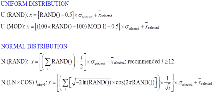 | Figure 1. Spreadsheet algorithms employed for the type of data set distribution generation with a selected mean and standard deviation |
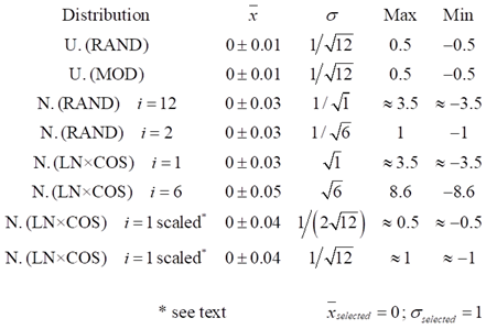
Table 1 collects some statistical parameters (mean, standard deviation and max and min values) for the different data sets generated with the algorithms described above. It can be seen that both algorithms for uniform distribution perform identically and produce the expected results, especially the standard deviations obtained. Both algorithms using the normal distribution also provide the expected results. The number of RAND times employed in the function is also shown in Table 1, showing their influence on the statistical parameters of the distributions. Thus, an increase in the use of the RAND function implies a higher value of the standard deviation and broader range for the extreme values max and min.Table 1. Selected statistics parameters for the different distributions generated
 |
| |
|
Figure 2 shows that it is hard to distinguish between the two types of distributions, uniform or normal, just by visual inspection of the sequence of values. The construction of a histogram creating a series of bins (class intervals) with an increment of 0.02 each and sorting values according to the intervals (bins) in which they occur, leads to the distributions shown in Figure 3. This operation can be easily performed in Excel by using the Data Analysis tool.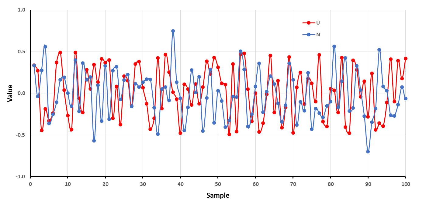 | Figure 2. Scattered values around zero obtained by using the uniform distribution function scaled between -0.5 and 0.5, U, and a normal distribution algorithm, N. Both have the same σ = 1/√12 |
Figure 3 shows the histograms for different types of distributions. The values for the uniform distribution (red bars) are random distributed showing no pattern, with their values perfectly confined between -0.5 and +0.5. Nevertheless the normal distribution (blue bars) with the same standard deviation, σ = 1/√12, produces the bell-shaped pattern, but there are values greater than 0.5 and below -0.5. These latter values account for approximately 5% of the entire set. The violet and green histogram are obtained for a normal distribution using RAND function and the Box-Muller transformation, both scaled to a standard deviation 1/(2√12), half of the blue histogram. Both histograms are independent of the algorithm employed. Moreover, with standard deviation value selected, less than 0.5% of the values lays outside of the -0.5/+0.5 interval. The selection of the distribution type and its scaling is our next task.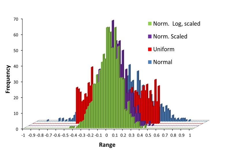 | Figure 3. Comparative histograms for different distributions, with zero as mean value. Red: Uniform, σ = 1/√12; Blue: Normal, σ = 1/√12; Violet: Normal, σ = 1/(2√12) and Green: Normal log based: σ = 1/(2√12) |
3. Analysis of the Influence of Noise Type on Linear Regression
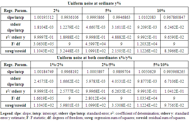
A common task performed by students is to create a plot from the data to extract information about a physical phenomenon. Among the different kinds of graphical analyses, linear regression is the most frequently encountered procedure. In order to analyze the influence of noise on the linear parameters, a controlled level of random noise has been introduced into the data along both coordinate axes. The amount of noise introduced at each data point is set to a selected percentage of the actual value, hence the new value fluctuates randomly around the original value.The uniform distribution provides easy control of the range of output values, and has here been set to vary between -0.5 and 0.5, so with a mean value of zero. Thus for each data point, a random percentage of fluctuation around its actual value can be added, employing the equation:  where, RAND(-0.5↔0.5), represents the algorithm to obtain a real number between -0.5 to 0.5 with a selected type of distribution. Thus, the percentage of noise is distributed randomly (under a uniform or normal distribution), around the actual value, adding or subtracting half the percentage of the noise selected.However, this procedure implies that the noise-free value zero is singular, i.e. it has no noise added using the above equation. Nevertheless, this can be remedied if an extra percentage of random noise is included for each data point as an offset, positive or negative, reducing this singularity. The amount of noise used to produce the offset is chosen at a level that is less by a factor of ten compared to the level of noise selected. As stated before, a normal distribution with the same standard deviation as the uniform one, produces values outside of those selected for the uniform distribution. Thus, to maintain approximately the same interval of values, the standard deviation of the normal distribution should be scaled, dividing by 1/(2√12) ≈1/7, as can be seen in figure 3, producing values that are more concentrated around the mean value. In this sense, when noise is injected using scaling of the normal distribution the actual values are less biased.All these different approximations for injecting noise in the data set have been tested and analyzed: uniform distribution, normal distributions with different standard deviation scales, and for each case, with and without additional offset. The analyses have been performed over a data set containing ten points that were generated using a simple linear relationship of the form y = x + 1. For each type of noise distribution, five different percentages of noise levels were injected: 0.5%, 1%, 2%, 5% and 10% for the ordinate and 0.2%, 0.5%, 1%, 2% and 5% for the abscissa. The sum over squared deviations varies approximately from 2·10-4, for 0.2% to 0.1 for 5% in the case of the uniform distribution applied to the abscissa and from 1·10-3 for 0.5% to 0.5 for 10% in the ordinate. When the correction for the singular noise-free value as mentioned above is applied, the values of the sum of squared deviations are very similar.Applying the scaled normal distribution, the values of the sum over squared deviations are approximately from 3·10-5, for 0.2% to 0.04 for 5% for the abscissa and from 2·10-4 for 0.5% to 0.1 for 10% for the ordinate. No significant changes are observed when a small offset is added to minimize the singular zero value. These values of the sum over squared deviations agree with the expected behavior, namely that noise generated by the uniform distribution will produce stronger fluctuations with poorer regression statistics than the scaled normal distribution.In order to analyze the influence of the kind of noise distribution and its level in both variables, linear regression statistics have been performed by means of the LINTEST routine in Excel.Table 2 summarizes, as an example, the results of a regression statistical analysis for the injection of different levels of uniform noise. The sub-table at the top reports results obtained when noise is added only to the ordinate values, while the lower sub-table gives LINTEST output when noise is added to both coordinates. The % level of noise injected is indicated in the column headers. Clearly, from the data in Table 2, lower noise added implies better statistics for the linear regression parameters (r2, std err, residual, and % relative error) indicative of a greater reliability of the model equation.
Table 2. Linear regression statistics by using the LINTEST function in Excel for different uniform noise levels added to the ordinate only and to both coordinates (x,y), respectively
 |
| |
|
Figures 4 and 5 show the relative error in the ordinate, and a close-up view of one point of the data set, (2, 3), respectively. Different levels of uniform distribution noise have been employed, in figure 4 only in ordinate and in figure 5 both coordinates. The shaded area in figure 5 approximately delineates the limits of the (x, y) fluctuation range.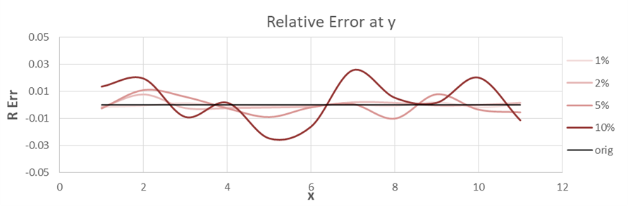 | Figure 4. Relative error associated with different percentages of uniform noise levels injected along the ordinate |
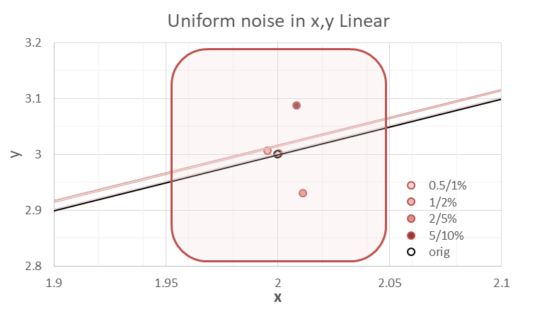 | Figure 5. Close-up view of the approximate area of fluctuation when different percentages of uniform noise levels are injected along both coordinates x, y |
An analysis of the % relative error in slopes, intercepts and regression residuals for the different levels of noise and for the different kinds of distributions has been performed. The results are summarized in 3D plot format for ease of comparison. Many plots of this type have been generated, and the ones shown here can be considered as typical for the general pattern.Figures 6, 7 and 8, show column diagrams for the relative errors in the slope, intercept and the squared sum of the regression residuals for Uniform (red) and Normal scaled (blue) distributions at different levels of noise for the ordinate only and for both coordinates. The % of noise is indicated in the plots. In general, the relative error in the intercept is approximately five times higher than that in the slope, noting the different scales in figures 6 and 7. Additionally, the error in the intercept increases when the extrapolation is made far from the data set interval. More often than not, when these calculations are repeated many times, it is more likely to obtain higher relative errors and regression residuals for the uniform than for the scaled normal distribution.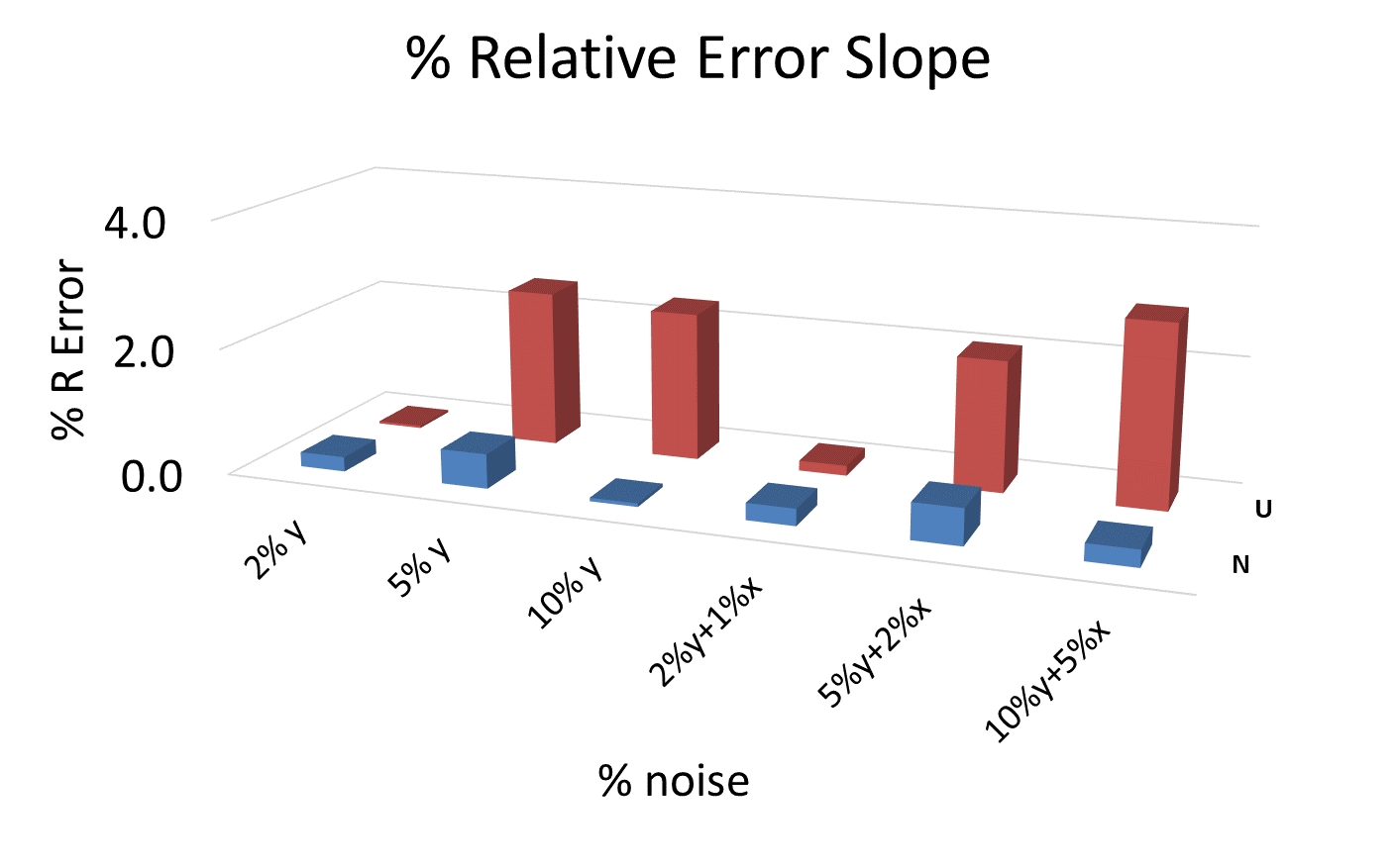 | Figure 6. Relative % error in the slope parameter for different noise levels and for both distributions, uniform (U) and normal (N) |
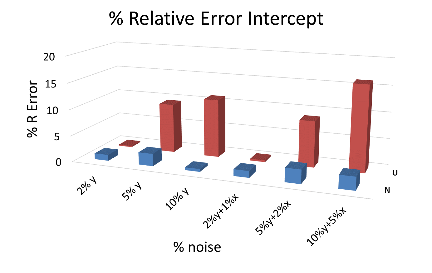 | Figure 7. Relative % of error in the intercept parameter for different noise levels and for both distributions, uniform (U) and normal (N) |
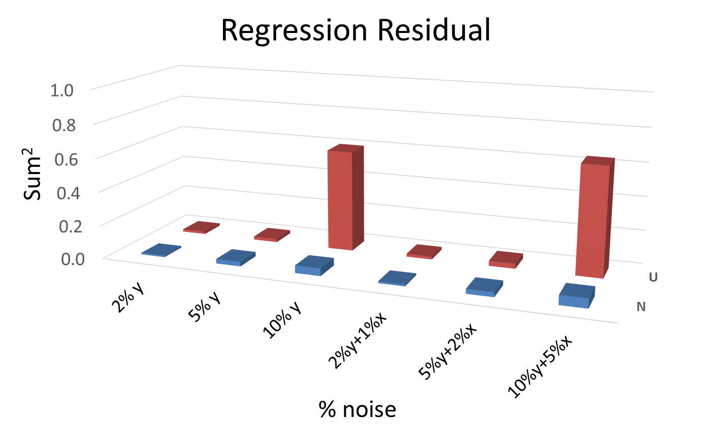 | Figure 8. Squared sum of the regression residuals for different noise levels and for both distributions, uniform (U) and normal (N) |
Generally, these conclusions are still valid when the comparison is made using the normal distribution without scaling with the uniform distribution. However, the error level using the normal distribution without scaling is higher and closer to that obtained using the uniform distribution. This behavior can be expected as extreme values under the normal distribution have relatively low probability.In conclusion, the injection of random noise into a data set can be useful for generating different data sets for use in online tests and virtual labs.
4. Examples of Injection of Controlled Random Noise
In this section, three kinds of experiments from the undergraduate Physical Chemistry lab will be employed as examples of the application of the strategy presented above.
4.1. Chemical Kinetics of the Fading of Phenolphthalein in Strong Alkaline Media under Pseudo-First Order Conditions
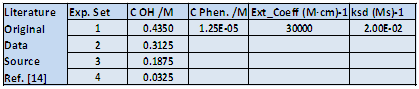
This is a classical experiment used for teaching chemical kinetics, involving the analysis of the change with time of the absorbance of a phenolphthalein solution at different high alkaline concentrations. The fading is second order overall, partial orders equal to one for each component, OH- and the Phenolphthalein anion. The goal is the determination of partial orders and the second order rate constant. This kinetic experiment has been part of our lab program for decades. It is advisable to perform the experiment at constant ionic strength by adding different concentrations of an inert salt. The general experimental conditions have been recently described [14], and reported results will be employed as initial data set.A new table is created in Excel from the data in table 3, by randomizing OH- concentrations, extinction coefficient and concentration of phenolphthalein and the second order rate constant. The kind and the % level of noise can be selected individually for each parameter. The goal is to add just enough noise to randomize the initial data set, while keeping the results obtained close to literature values, with a tolerance level of 20% being advisable. Taking into account that Excel randomizes the cell contents each time a cell is modified at any position on the worksheet, it is required to copy these generated values elsewhere on the worksheet. In this way the new data remain fixed for the rest of the calculations. This final table can be considered to be the data set corresponding to the results of a lab experiment.Table 3. Excel table containing the initial experimental conditions and literature data for the kinetics of phenolphthalein fading. The ionic strength is maintained at 0.435M
 |
| |
|
A new worksheet is generated containing the absorbance values for the four alkaline concentrations for different sampling times, by using the equations depicted in figure 9. These absorbance values, in our case, are randomized with a new percentage of noise, to mimic the possible fluctuations of the absorbance during the actual measurement process. In the original lab experiment, the absorbance is automatically read every second, and the reaction is monitored for 5 min.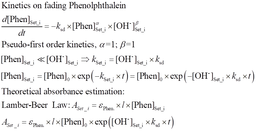 | Figure 9. Equations employed in the kinetic study of the fading of phenolphthalein. The symbols have their usual meanings |
This worksheet, together with the literature data for the initial concentrations and molar extinction coefficient, are the randomized data to be supplied online to students individually as an Excel file. Alternatively, if the examination is carried out face-to-face, as in a seminar, those absorbance values can be sampled, via Excel Data Analysis, to obtain a randomized small set of absorbance data that can be readily provided to the students.Figure 10 shows a screenshot of the Excel output when 20% Gaussian scaled noise is injected into the absorbance values. Initially the absorbance is generated using primary data with 10% noise level injected. As can be seen, even with a high level of noise injected, it is still possible to obtain values close to those reported in literature. Thus, this experimental design is very robust and useful for teaching chemical kinetics.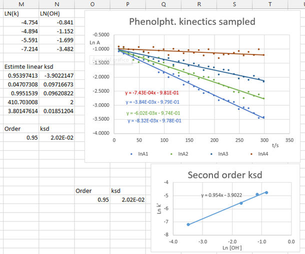 | Figure 10. Screen shot displaying the kinetics analysis results. 20% noise error added absorbance data |
4.2. Estimation of the Limiting Molar Conductivity of an Electrolyte Based on Kohlrausch’s Law
Obtaining the infinite dilution molar conductivity of an electrolyte is another classical experiment in the Physical Chemistry teaching lab. The experiment is easily carried out with a cheap portable conductivity meter. In this case the students have to obtain a linear Kohlrausch’s relationship between the molar conductivity and the square root of the electrolyte concentration and from the intercept at zero concentration, the limiting molar conductivity of the electrolyte is obtained. The comparison with literature data offers information about student’s skills in preparing solutions and their glassware-cleaning protocols. The experimental data are the specific conductivities of the electrolyte solution. The specific conductivities of the most dilute solutions have to be corrected for the contribution from the solvent, usually water. The initial data set for different true electrolytes are culled from the literature, [15]. Another possible approach is to generate the data from the Debye-Hückel-Onsager equation, knowing the limiting molar concentration and the constants A and B, see figure 11.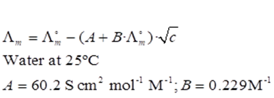 | Figure 11. Debye-Hückel-Onsager equation and parameters A, B, for water at 25°C |
A set of initial values of molar conductivities at different concentration is selected, in our case, KNO3, K2SO4, KIO3 and sodium oxalate. These concentrations can be randomized to obtain the different molar conductivities. From them, a set of randomized specific conductivities can be generated. For this case, uniform distribution-type noise has been selected. The experimental concentration range is usually from 10-4 M to 10-2 M, but can be modified. The specific conductivity for low electrolyte concentrations has to be corrected for the water contribution, and this can be another source of randomization.The randomization process is analogous to that used in the kinetics experiment. A worksheet contains the initial data, and from these the randomized set is generated. Figures 12 and 13 show the literature data of Kohlrausch’s plots for the selected salts and those recalculated after randomization, respectively.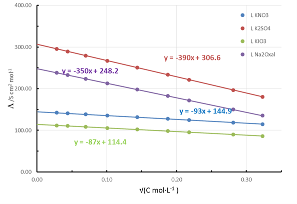 | Figure 12. Literature-generated Kohlrausch plots for different selected salts |
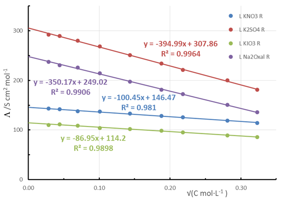 | Figure 13. Estimated Kohlrausch plots for different salts after randomization produced by adding 5% of uniform noise to the literature data |
In this case, a low level of noise should be injected because the parameter of interest is obtained from the intercept, the one most sensitive to higher noise levels, as was illustrated earlier. Nevertheless, with this noise level in combination with literature information, many randomized data sets can be constructed. This strategy can be applied also to obtain the limiting conductivity for a weak electrolyte and its dissociation equilibrium constant. In this case, the parameters are obtained by extrapolating far from the data set interval. Consequently, special care should be taken in choosing the level and type of noise to be injected.
4.3. Estimation of the Enthalpy of Vaporization Based on the Clausius-Clapeyron Equation
The determination of the enthalpy of vaporization of water constitutes another standard lab experiment in the Physical Chemistry lab. The typical experiment is based on the measurement of the change of the water vapor pressure with temperature when the vapor and the liquid water phases are in equilibrium. The results are analyzed by using the approximate Clausius-Clapeyron (CC) expression, where the molar volume of water is neglected with respect of that of the liquid, the enthalpy of vaporization is independent of temperature and ideal gas behavior is assumed for the water vapor [16].The CC equation can be formulated for the liquid/vapor equilibrium: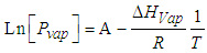 where Pvap is the water vapor pressure, A is a constant, ΔHvap is the molar enthalpy of vaporization of water, assumed to be constant in the temperature range considered, R the gas constant and T the temperature in K. In our lab, a distillation glassware system containing water which can be heated and is connected to a vacuum pump is employed. A simple three-way manually operated valve allows easy control of the pressure in the system. The arrangement permits the measurement of vapor pressure (Pvap) and the temperature (T) data at equilibrium, from room temperature to the normal boiling point.Figure 14 shows the linear plots (ln Pvap vs. 1/T) according to the CC equation obtained by three students with different levels of laboratory skills. As can be noted, the degree of data scatter is higher for lower temperatures, where equilibrium conditions are less easy to attain.
 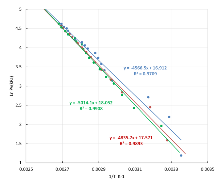 | Figure 14. Experimental Clausius-Clapeyron plots based on data, independently obtained by three undergraduate students |
Literature data [15], obtained as Pvap vs t/°C, for the phase equilibrium between water vapor/liquid at the conditions prevailing in the lab (25°C-100°C) are plotted as a CC linear plot in Fig. 15.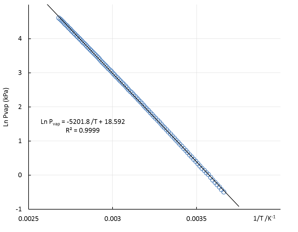 | Figure 15. Water vapor/liquid equilibrium Clausius-Clapeyron plot from literature data [15] for the temperature range employed in the lab |
Notwithstanding the good linear relationship, slight differences between the data points and the straight line can be noted specially for the two temperatures limits. This is another sign of the accuracy of the assumptions used in applying the CC equation.Taking into account all these considerations, the controlled injection of noise has been applied to generate randomized Pvap/T data from literature sources. Both types of noise have been injected, the Uniform and the Normal (log based, scaled). Different levels of noise have been applied to the experimental variables: vapor pressure in kPa and temperature in Celsius scale, ranging from 10% to 40% for Pvap and 1% to 5% for temperature. The logarithmic character for the ordinate variable in the CC equation, in addition to the fact that the parameter of interest is obtained from the slope, permit high levels of noise for the vapor pressure. This fact ensures the successful performance of these experiments in the undergraduate lab. The heat of vaporization obtained by a moderately skilled student is always close to the literature value, boosting student’s self-confidence. Nonetheless, the level of noise applied to temperature values has to be controlled carefully to obtain significant results, and a maximum fluctuation range of 5% is recommended. Figure 16, shows the influence of noise injection in the sampled literature data from Fig. 15. The same conclusions reached in section 3 apply here. Injection of uniform noise produces poorer linear regression parameters than the normal scaled noise at the same percentage level. Even though randomized Gaussian noise produces an outlier, the slope obtained is close to the literature data. The occurrence of these outlier values in a data set is not very likely. The slopes obtained from plots with injected Gaussian noise are likely to end up closer to the literature value than those obtained with uniform noise.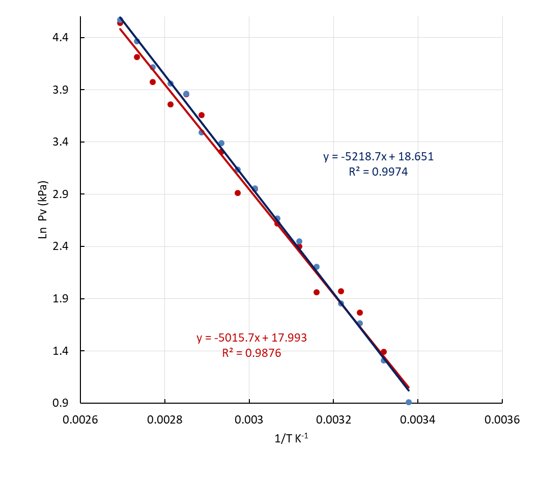 | Figure 16. Clausius-Clapeyron plots obtained by injecting to literature data Uniform- and Normal- (log based, scaled) type noise, with a 40% range for Pvap in kPa and 5% for temperature in °C |
5. Conclusions
In conclusion, some recommendations can be implemented for randomized data sets by using injection of noise. First, the application of noise has to be carefully controlled, that is, the results obtained from the analysis of the noisy data set have to be realistic and reliable. For each specific situation and set of conditions, a check should be performed prior to selecting the appropriate amount of noise. Secondly, it is advisable to use uniform (white) noise for data sets that already contain natural random noise, such as the data sets culled from literature. And finally, normal distribution (Gaussian) noise should be employed for data sets generated directly from theoretical or simulated equations, producing noisy data sets that have a more natural appearance.
ACKNOWLEDGEMENTS
The authors are indebted to M. A. Guerra Aguilar-Galindo for his continuous, deep involvement with and dedication to the Labs of the Physical Chemistry Dpt. of the University of Seville.
References
| [1] | Blackboard online EdTech, Learning Platform homepage. [Online]. Available: https://www.blackboard.com/. Accessed April 2021. |
| [2] | Collaborative Learning Management System. Learning platform homepage. [Online]. Available: https://moodle.com/. Accessed April 2021. |
| [3] | ChemCollective Resources homepage. [Online]. Available: http://chemcollective.org/home. Accessed April 2021. |
| [4] | Virtual Chemistry homepage. [Online]. Available: http://www.chem.ox.ac.uk/vrchemistry/. Accessed April 2021. |
| [5] | Virtual Labs homepage. [Online]. Available: https://www.labster.com. Accessed April 2021. |
| [6] | Virtual Chemistry and Simulations homepage. [Online]. Available: https://www.acs.org/. Accessed April 2021. |
| [7] | S.W. Smith, “The Scientist and Engineer's Guide to Digital Signal Processing”, 1999, 2sd Ed., California Tech. Pub. USA. |
| [8] | W.H. Press, S.A. Teukolsky, W.T. Vetterling and B.P. Flannery. “Numerical recipes. The art of Scientific Computing” 2008, 3rd Ed. Cambridge U. Press. Cambridge, UK. |
| [9] | M. Matsumoto and T. Nishimura, (1998). "Mersenne twister: a 623-dimensionally equidistributed uniform pseudo-random number generator" Mersenne Twister MT19937 (32bits). ACM Transactions on Modeling and Computer Simulation. 8 (1): 3–30. CiteSeerX 10.1.1.215.1141. doi: 10.1145/272991.272995. S2CID 3332028. |
| [10] | E.W. Weisstein, "Uniform Distribution." From MathWorld--A Wolfram Web Resource. [Online]. Available: https://mathworld.wolfram.com/UniformDistribution.html. Accessed April 2021. |
| [11] | I. Niven, “Uniform Distribution of Sequences of Integers”, Transactions of the American Mathematical Society, 1961, Vol. 98, No. 1, 52-61. |
| [12] | Y. Dodge, 2008, “The Concise Encyclopedia of Statistics”. Springer, New York, NY. https://doi.org/10.1007/978-0-387-32833-1_50. |
| [13] | E.W. Weisstein, "Box-Muller Transformation." From MathWorld -- A Wolfram Web Resource [Online]. Available: https://mathworld.wolfram.com/Box-MullerTransformation.html. Accessed April 2021. |
| [14] | D. González-Arjona, M. M. Domínguez, G. López-Pérez and W. H. Mulder. “Primary Kinetic Salt Effect on Fading of Phenolphthalein in Strong Alkaline Media: Experimental Design for a Single Lab Session” The Chemical Educator. 2019, vol. 24, 126-132. |
| [15] | W. M. Haynes, Lide, D. R., & Bruno, T. J. Ed., CRC handbook of chemistry and physics: a ready-reference book of chemical and physical data. 2016-2017, 97th Edition, CRC Press. |
| [16] | P.A. Atkins, J. de Paula and J. Keeler. “Atkins' Physical Chemistry”, 2017. 15th Ed. Oxford U. Press. Oxford. |

 Abstract
 Reference
 Full-Text PDF
 Full-text HTML