Mine Ucak-Astarlioglu1, Sarah Edwards2, Christopher A. Zoto3
1Department of Chemistry, The George Washington University, Washington, DC, U.S.
2Department of Chemistry, Western Kentucky University, Bowling Green, KY, U.S.
3U.S. Army Natick Soldier Research, Development, and Engineering Center, Natick, MA, U.S.
Correspondence to: Christopher A. Zoto, U.S. Army Natick Soldier Research, Development, and Engineering Center, Natick, MA, U.S..
| Email: |  |
Copyright © 2017 Scientific & Academic Publishing. All Rights Reserved.
This work is licensed under the Creative Commons Attribution International License (CC BY).
http://creativecommons.org/licenses/by/4.0/

Abstract
The experiments presented in this manuscript provide undergraduate students with valuable exercises in experimental and computational physical chemistry and a clear understanding to the characterization of the physical and chemical properties of chemical compounds. Spectroscopic studies of two commercially available -conjugated organic dyes, namely sulforhodamine B and malachite green, were examined experimentally and computationally. UV-Visible absorbance and fluorescence spectra of both compounds were measured in solvents of various polarity. It was found that sulforhodamine B is a more red shifted dye than malachite green, in that it absorbs and fluoresces strongly in the red region of the visible spectrum, contrary to malachite green, which is a blue shifted compound. The absorbance and fluorescence spectral maxima locations are clearly indicative in the colors of these compounds in solution. In addition to measuring experimental spectra, quantum chemical calculations were also performed using Spartan and Gaussian, calculating and visualizing molecular orbital coefficients and molecular orbitals.
Keywords:
Physical Chemistry, Dyes, Spectroscopic, Absorbance, Fluorescence, Molecular Orbitals
Cite this paper: Mine Ucak-Astarlioglu, Sarah Edwards, Christopher A. Zoto, Spectroscopic Properties of Two Conjugated Organic Dyes: A Computational and Experimental Study, Journal of Laboratory Chemical Education, Vol. 5 No. 2, 2017, pp. 32-39. doi: 10.5923/j.jlce.20170502.04.
1. Introduction
In chemistry, and in physical chemistry particularly, experimentation is crucial for students to understand the concepts of constructing theories. In the current scientific world, analytical instrumentation (i.e. spectrophotometers) and computational software programs (i.e. Mopac, Gaussian, and Spartan) are heavily used for the characterizations of compounds. Computational chemistry is a crucial bridge between experiments and theory. Because of this reason, more computational chemistry related experiments that are correlated to the experimental work need to be incorporated into physical chemistry laboratory courses. The work presented in this manuscript provides a short presentation and discussion of the spectroscopic properties of two -conjugated organic compounds, namely sulforhodamine B and malachite green (chemical structures shown in Figure 1). This work serves as an educational tutorial for students to better understand the connection between experimental physical chemistry and computational chemistry. Sulforhodamine B and malachite green were chosen due to the presence of their different electron donor/acceptor functional groups, planarity, rigidity, and absorbance and fluorescence properties. Previous work published in the Journal of Chemical Education by Ucak-Astarlioglu and coworkers [1] involved studying the optical properties of cadmium selenium (CdSe) quantum dots, or semiconductor nanocrystals, and this work was published as a laboratory experiment intended for undergraduate level chemistry students. The absorption and fluorescence spectra of solutions of mixtures of the quantum dots and organic fluorophore dyes (of the coumarin and rhodamine series) were measured.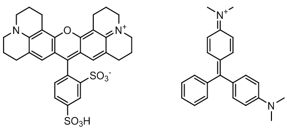 | Figure 1. Chemical structures of sulforhodamine B (left) and malachite green (right) |
Previous work studying the structural and spectroscopic properties of a series of unsubstituted and substituted 2-arylidene and 2,5-diarylidene cyclopentanone compounds serves as background for this experiment [2-6]. Cited studies show that these classes of organic compounds undergo bathochromic (red) shifts with respect to increased solvent polarity, some more pronounced than others. In general, the compounds containing stronger electron donor and acceptor groups were found to undergo more significant bathochromic shifts, larger Stokes’ shifts, and exhibit photoinduced internal charge transfer properties. In internal charge transfer, photoexcitation causes the electron density to be transferred within the molecule, from the electron donor end of the molecule in the Highest Occupied Molecular Orbital (HOMO) to the electron acceptor end of the molecule in the Lowest Unoccupied Molecular Orbital (LUMO). The computational component of this project involved performing molecular orbital and molecular orbital coefficient calculations using Gaussian 03 and Spartan.The laboratory experiment presented in this manuscript was performed in a once per week three hour lecture/lab course in a Physical Chemistry Lab at Penn State University and also in an Instrumental Chemistry Lab at George Washington University. This experiment can be used in advanced level undergraduate or beginner level graduate chemistry laboratory courses as a regular laboratory experiment in physical chemistry, instrumental chemistry, computational chemistry, and analytical chemistry laboratories. Students were asked to do literature searches on the dyes, instrumentation, and application of computational chemistry in electronic structure determination as part of the project. Tutorials were posted online for learning and using software packages, instrumentation, and solution preparations. Each week, students had the option of attending one-on-one or group-based office hours with the instructor. Each group consisted of four students. Each group was asked to work together on tasks distributed by the instructor as part of the lesson plan. A total of 16 students from both universities obtained successful results from this experiment and discussed their findings in oral and written scientific language.Presented in the experimental part of this manuscript are the types of chemicals, analytical instrumentation, and computational software that were used in the experiments. Please refer to the Supplementary Information at the end of the manuscript, which provides the necessary laboratory documentation and the step-by-step procedures of both the experimental and computational components of this project.
2. Experimental
Sulforhodamine B (MP Biomedicals) and malachite green (Fisher Chemical) were used as is without further purification. All solvents except ethanol were of spectral grade purity purchased from Acros Organics. Ethanol (ethyl alcohol, 200 proof) was purchased from Pharmco-AAPER. A Thermo Scientific Evolution 600 UV-Vis Spectrophotometer was used to measure the room temperature UV-Visible absorbance spectra and a Horiba Scientific FluoroMax-4 Spectrofluorometer was used to measure the room temperature fluorescence spectra. The proper Personal Protective Equipment (PPE) was used for all chemical handling, solution preparations, and spectroscopic measurements in accordance to the Safety Data Sheets (SDS’s). Both Spartan and Gaussian 03 were used to perform all quantum chemical calculations. The molecular geometries of both compounds were optimized using Spartan [7, 8]. From the output file, the Cartesian coordinates were saved and extracted for use as Gaussian input files [9, 10]. From the optimized geometries, molecular orbital calculations ran in parallel; that is, Spartan was used to calculate the molecular orbitals and provide the visual images of the computed HOMOs and LUMOs [7, 8]. Gaussian was used to calculate the specific molecular orbital coefficients [9, 10].In the first 30 minutes, students had the lab course in lecture style. In the second half of the hour, students had the laboratory session. During the first week, in the lecture part, the instructor presented the dyes, talked about the molecular and electronic structures of the dyes, and the chemical instrumentation and experimental techniques in analyzing and determining the spectroscopic properties of the dyes. For the remainder of the laboratory period, students were allowed to prepare the solutions and conduct spectroscopic measurements on both the UV-Visible absorption and fluorescence spectrometers.During the second week, in the lecture part, students were allowed to draw the structures of the chemical compounds and were introduced to computational calculations. Students were trained on the importance of using quantum chemistry in determining the electronic structure differences in the dyes. During the rest of the laboratory period, students continued work on the spectroscopic measurements. During the third week, students completed all remaining experiments and worked on completion of their papers and presentations. At both Penn State University and George Washington University, student presentations were given to the Chemistry Department audience including faculty, graduate, and undergraduate students at the end of the semester, which was integrated in part of their grading.
3. Results and Discussion
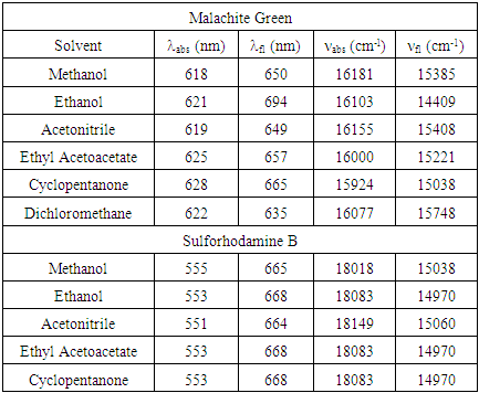
Experimental UV-Visible Absorbance and Fluorescence SpectraTable 1 lists the UV-Visible absorbance and fluorescence spectral maxima locations of sulforhodamine B and malachite green in the studied solvents. It was observed that only a minor degree of solvatochromic shifting was observed in the absorbance spectra, with net spectral shifts of 10 nm (ν 257 cm-1) and 4 nm (ν 90 cm-1) for malachite green and sulforhodamine B, respectively. In fluorescence, only a small degree of shifting was observed for sulforhodamine B (λ 4 nm, ν 90 cm-1). However, a larger degree of shifting was observed in the fluorescence of malachite green. It was found that malachite green underwent a net bathochromic shift of 59 nm (ν 1339 cm-1) in going from dichloromethane to ethanol. Figure 2 shows the sets of UV-Visible absorbance spectra of malachite green and sulforhodamine B in all solvents studied. Figure 3 shows the sets of fluorescence spectra of malachite green and sulforhodamine B in all solvents studied.Table 1. Absorbance and fluorescence spectral maxima of malachite green and sulforhodamine B in all studied solvents
 |
| |
|
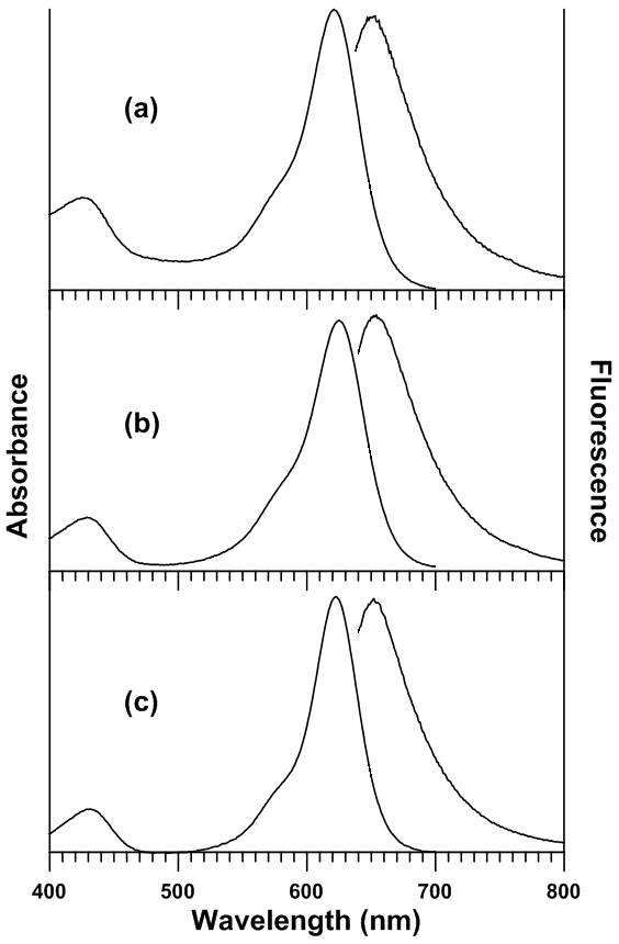 | Figure 2. UV-Visible absorbance and fluorescence spectra of malachite green in (a) ethanol, (b) ethyl acetoacetate, and (c) dichloromethane |
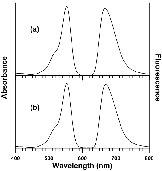 | Figure 3. UV-Visible absorbance and fluorescence spectra of sulforhodamine B in (a) ethanol and (b) ethyl acetoacetate |
The higher degree of red shifting observed in the fluorescence of malachite green, contrary to sulforhodamine B, is most likely attributed to the presence of free moving, or labile, electron donor/acceptor groups on the aryl moieties. Malachite green contains free-moving dimethylamino groups substituted on the aryl moieties that can potentially undergo the formation of a twisted internal charge transfer (TICT) state. A TICT state is a special type of internal charge transfer state, where, in the case of malachite green, the plane of the dimethylamino group is at a twisted angle with respect to the rest of the molecule due to rotation about the C-N bond. TICT states form in highly polar solvent environments (i.e. alcohols) and their fluorescence is quenched and red shifted relative to the locally excited state. Sulforhodamine B is spatially restricted on the aryl moieties due to the presence of closed, saturated ring systems that structurally prevent it from having a TICT state. Another interesting observation to note is that sulforhodamine B is orange and red in solution, whereas malachite green is green in solution (see Figure 4). The differences in the color are due to the wavelength regions in the visible spectrum that these compounds absorb and emit strongly at.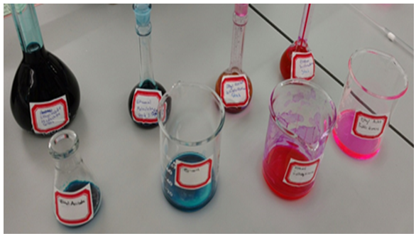 | Figure 4. Solutions of malachite green (left four) and sulforhodamine B (right four) prepared |
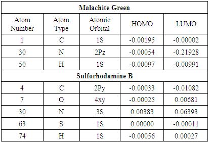
Quantum Chemical CalculationsTable 2 presents a selection of computed molecular orbital coefficients of atom/orbital pairs for malachite green and sulforhodamine. To reiterate, the molecular orbital coefficients indicate how much a given atomic orbital contributes to the overall molecular orbital. Table 2. A selection of computed molecular orbital coefficients of atom/orbital pairs for malachite green and sulforhodamine B
 |
| |
|
The visual representations of the HOMOs and LUMOs are shown in Figure 5. In these representations, the red and blue shaded areas represent regions of electron density with the two different phases of the orbitals. By looking at the visual representations of the HOMOs and LUMOs, it is possible to see the regions of greater electron density around more electronegative atoms, such as nitrogen, and in π-bonding regions. Because sulforhodamine B has an unequal number of α and β electrons, something determined by counting the electrons in the Lewis structure and following Hund's rule to figure out which orbitals they fill, it has α and β HOMOs and LUMOs Malachite green has equal numbers of α and β electrons, and as such only have one HOMO and one LUMO. The energy difference between the HOMO and the LUMO (the HOMO/LUMO gap) is a key factor in determining fluorescence activity and these calculations are the first step in much more complicated calculations to be undertaken in the future. 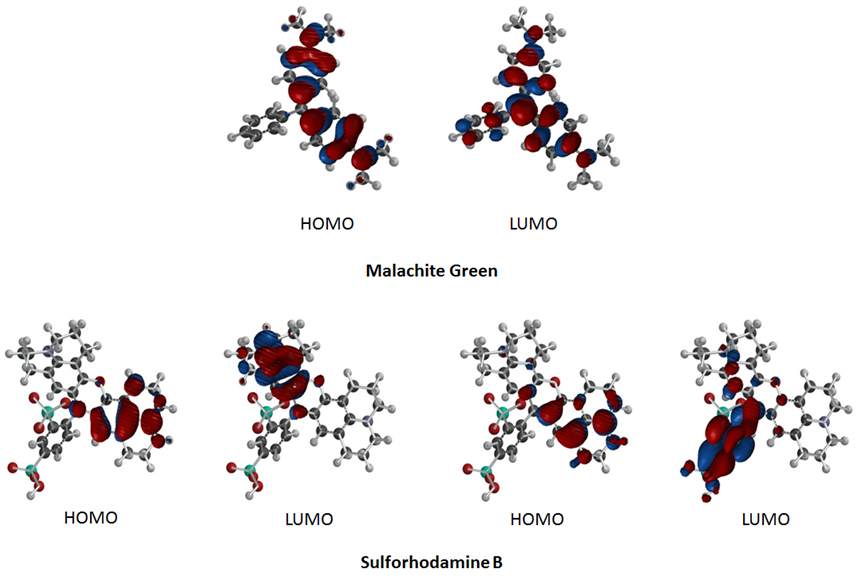 | Figure 5. Computed HOMOs and LUMOs of malachite green and sulforhodamine B |
4. Conclusions
The spectroscopic properties of two conjugated organic dyes, namely malachite green and sulforhodamine B, were studied both experimentally and computationally. Room temperature UV-Visible absorbance and fluorescence spectra were measured in solvents of different polarity. It was found that both compounds exhibited minor degrees of solvatochromism in their absorbance spectra. In fluorescence, however, minor solvatochromism was observed for sulforhodamine B and a higher degree of solvatochromism was observed in malachite green. The higher degree of bathochromic (red) shifting observed in the fluorescence of malachite green is most likely attributed to the production of a TICT excited state, which is more red shifted relative to the locally excited state. On a structural standpoint, malachite green contains free moving, or labile, dimethylamino groups that can undergo twisting about the aromatic rings; however, sulforhodamine B cannot due to the presence of closed, saturated ring systems that structurally prevent it from having a TICT state. Computational characterization involved carrying out geometry optimizations, molecular orbitals, and molecular orbital coefficient calculations. On an educational standpoint, the work presented in this manuscript exposes the student with valuable exercise in experimental and computational physical chemistry. In the laboratory environment, students get hands on experience running experimentally observed work and collecting data, of which they can directly compare to theoretically predicted (computational) data. Computational calculations should be started ahead of time for a timely completion of results, which can range from single or multiple days, depending on the molecular structures, levels of theory/basis sets used, and the types of calculations.
ACKNOWLEDGMENTS
We would like to respectfully acknowledge Dr. Gail Clements, Dr. Michael King, and Amanda Egan from George Washington University and Drs. Mark Maroncelli, Josh Sokoloski, Minjoung Kyoung, and Ajeet Kumar from Penn State University for making this experiment a viable one for Instrumental Analysis and Physical Chemistry labs, respectively. Authors would also like to thank to the students of Georgetown University/Instrumental Analysis Labs for conducting spectroscopic analysis, and students of Penn State University/Physical Chemistry Labs for conducting spectroscopic and computational analyses of the dyes under investigation.
Supplementary Information
Laboratory Documentation1. Background1.1. SolvatochromismSolvatochromism is the ability of a chemical substance to change color in different solvents (1, 2). Depending upon the nature of the solvent environment, solvatochromic molecules undergo either hypsochromic (blue) shifts or bathochromic (red) shifts in their optical absorption and fluorescence spectra. Hypsochromic (blue) shifts are spectral shifts to shorter wavelengths or higher energies and bathochromic (red) shifts are spectral shifts to longer wavelengths or smaller energies. From previous work done in our lab, we found that (2E,5E)-2,5-bis(4-dimethylaminocinnamylidene) cyclopentanone exhibited a larger degree of solvatochromism, as illustrated in Figure 1, in that its color changes from yellow à orange à red à purple with respect to an increase in solvent polarity (3). 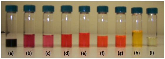 | Figure 1. Solutions of (2E,5E)-2,5-bis(4-dimethylaminocinnamylidene) cyclopentanone in (a) 2,2,2-trifluoroethanol, (b) ethanol, (c) 2-propanol, (d) acetonitrile, (e) acetone, (f) ethyl acetate, (g) benzene, (h) toluene, and (i) cyclohexane |
1.2. Quantum MechanicsComputational methods rely on the approaches and theorems of quantum mechanics, which uses electrons as the basis of chemistry. Electrons do not exist at discrete points around the nucleus. Rather, they each exist in a region of probability defined by the wavefunction of the given electron, denoted as ψ. This electronic wavefunction is found by the solution of the Schrodinger equation Eq. 1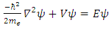 | (1) |
where  is Reduced Planck's constant, which is equal to Planck’s constant (6.626 x 10⁻³⁴ J s) over 2π, me is the electron rest mass (9.11 X 10⁻³¹ kg),
  is the Laplacian operator, defined as the sum of the second order partial derivatives with respect to all coordinates, V is the potential energy felt by the electron, and E is the total energy of the system (4). When coupled with the spin of the electron, α or β, these one electron wavefunctions become atomic orbitals and can further overlap to form molecular orbitals from the Linear Combination of Atomic Orbitals to form Molecular Orbitals (LCAO-MO) (see Figure 2).
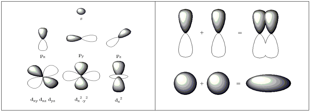 | Figure 2. Depiction of the various s, p, and d atomic orbitals (left) and an illustration of the linear combination of atomic orbitals to form molecular orbitals (right) |
The overall wavefunction for a multi-center multi-electron system is defined by Eq. 2  | (2) |
where the subscripts denote the number of the atomic orbitals and the letters within the parentheses represent the atoms to which the atomic orbitals belong to. The coefficients c in front of each atomic orbital are called the molecular orbital coefficients and are directly proportional to the contribution of each atomic orbital to the overall molecular orbital (4). The molecular orbital wavefunctions are only useful within the Born-Oppenheimer Approximation, which is an approximation method in quantum mechanics for multi-center multi-electron systems that discusses the electron motion and location within the field of stationary nuclei (5), referred to as LCAO-MO.Molecular orbitals, like atomic orbitals follow Hund's Rule, which states that electrons must occupy orbitals of lower energy before orbitals of higher energy. The HOMO and the LUMO are of particular interest because the energy gap between these two molecular orbitals describes oxidation potentials, ionization energies, absorbance and fluorescence spectral properties, and reactivity. In the case of unequal numbers of α and β spin electrons, there are two different HOMOs and LUMOs, α and β, which correspond to α and β spin orbitals (6). 1.3. Computational Chemistry Computational methods, by modeling these wavefunctions, are used to calculate the molecular orbital coefficients of multi-electron systems. The Schrodinger equation is straightforward for the one electron system, yielding a solution defined by the wavefunction defined in Eq. 3.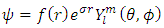 | (3) |
where r is the electron distance from the nucleus,  is the charge over the Bohr radius, f(r) is unique to each atomic orbital, Y is the angular dependence of the orbital, l is the azimuthal or orbital angular momentum quantum number, and m is the magnetic quantum number (4).For different quantum numbers, Eq. 3 becomes the familiar s, p, d, etc. orbitals as presented in Figure 2. It is difficult to work with systems where there is more than one electron present because the electron-electron interaction terms in the potential function result in complications in the solution of Schrodinger’s equation. To overcome these complications, approximations for the wavefunction, also known as a basis set, and potential functions are needed. In modeling the wavefunction of the multi-center multi-electron system, Gaussian functions are employed as given in Eq. 4
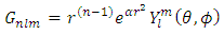 | (4) |
where α is specific to each atomic orbital and maximizes the overlap between the Gaussian function and the atomic orbital. The remaining terms are the same as given in Eq. 3. With the use of Gaussian functions, the problem is significantly simplified. This approximation works quite well for values of r greater than the Bohr radius; however, Gaussian functions and atomic orbitals behave very differently for small values of r, causing problems with molecular orbital calculations (4). Using a sum of Gaussian orbitals fit to match the atomic orbital is a solution which greatly increases the accuracy of the calculations. For example, using three Gaussians to estimate a 1s orbital gives Eq. 5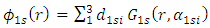 | (5) |
where  is the weight that each different Gaussian function carries in the sum. When sums of Gaussian functions are used, the accuracy of the calculation increases with respect to an increasing number of functions. However, one drawback is that each orbital of the same type described by this system will be the same size. The result being that a 1s and a 2s orbital will be the same size. To allow orbitals of the same type to be different sizes, a weighted sum of Gaussian functions with different
  the double zeta basis set Eq. 6 can be used.
 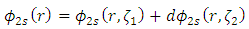 | (6) |
where  is the weighting term. A single zeta basis set is sufficient for inner core electrons, while a double zeta basis set better describes the valence electrons (4). This is known as a split valence double zeta basis set. For example, a 6-31G basis set is a split valence, double zeta basis set with 6 Gaussian functions describing the inner core electrons and three small and one large Gaussian function describing the outer valence electrons. It is important to note that these are all one electron wavefunctions. Creating multiple electron wavefunctions for multiple electron systems is as simple as multiplying the one electron wavefunctions, as shown in Eq. 7.
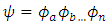 | (7) |
However, working with such equations is still not very straightforward because of the electron-electron interaction terms in the potential function. To overcome the complicated potential function problem, Hartree-Fock Theory is employed. Hartree-Fock Theory is an iterative process that makes an initial guess at which orbitals are filled (i.e. identification of the molecular orbital coefficients) and solves for the average potential felt by the electrons. This average potential is then used to solve for a new set of orbitals. The process is repeated until the potential and molecular orbital coefficients no longer change with iteration. The bottom line with Hartree-Fock Theory is to treat a complicated system of multiple electron-electron interactions as an average potential and reduce it to a one electron problem (7).2. Experimental Componenta. Solution PreparationIn a small glass vial (i.e. 10 mL), add 5 mL of the spectroscopic grade solvent. Using a glass Pasteur pipette, transfer a “tip” amount of the compound (from the pipette) into the glass vial containing the solvent. Gently swirl the pipette tip such that the solid is transferred into the solvent and goes into solution. Wait for about 15 minutes, then filter the solution by gravity filtration, collecting the filtrate. The way to gravity filter out the small volume-sized solutions is by taking a small piece of cotton wool and pushing the cotton down towards the tip until it cannot be pushed down any further. Then, with another glass pipette containing the unfiltered solution is added to the pipette containing the cotton wool. The filtrate is collected from the bottom of the pipette into a clean glass vial. At this point, a concentrated filtered solution of the compound in the solvent of interest has been prepared. b. Spectroscopic AnalysesQuartz (glass) cuvettes are required for measuring UV-Visible absorbance and fluorescence spectra since organic solvents are being used. It is important to pre-rinse the cuvette, first with acetone and then with the solvent of interest to avoid solvent cross contamination. Once this is done, then fill the cuvette ~ 3/4 to the top with the pure solvent of interest, and add filtered solution to the top of the cuvette. Pipette the ‘now diluted’ solution up and down a few times to ensure that it is completely mixed in with the pure solvent.When measuring the UV-Visible absorbance and fluorescence spectra, run the baseline first with only pure solvent. Once the baseline has been run and corrected, then the sample absorbance and fluorescence spectrum is measured. In the UV-Visible absorbance spectrum the maximum absorbance intensity (ODmax) value should max out between 0.5-1, respectively. If the ODmax does not lie within this range, it should either be diluted or concentrated appropriately, depending on the analyte concentration. The solution is diluted or concentrated appropriately in the cuvette. Once the UV-Visible absorbance spectrum is measured and collected for an ODmax between 0.5-1, use the peak pick labeler in the software to obtain the wavelength of maximum absorbance  Once the sample UV-Visible absorbance spectrum has been measured, the same solution is transferred to a 4 clear-walled quartz cuvette and the fluorescence spectrum is measured, fixing the excitation/absorbance wavelength at the
  obtained from the absorbance spectrum, scanning the fluorescence from
  nm to 900 nm (or 800 nm if the upper wavelength detection limit in the fluorimeter is not 900 nm). Once the fluorescence spectrum is measured, the software is used to obtain the wavelength of maximum fluorescence.Lastly, both data sets (absorbance and fluorescence) as well as the spectrum file format and the raw data format (format type is either .csv or .asc). The raw data can be copied and pasted onto an external graphing software like Microsoft Excel® or Grapher® to re-construct the spectra. All the raw data and plotted graphs are submitted to the instructor.3. Computational Component3.1. Student Information3.1.1. IntroductionComputational chemistry is a subset of theoretical chemistry. The purpose behind computational chemistry is to create useful mathematical approximations of molecules that have the capability to predict the physical properties of molecules. The purpose of this experiment is to develop a breadth of knowledge with regards to various current computational methods and capabilities. You will determine the HOMOs and LUMOs of malachite green and sulforhodamine B. Due to the resources required to create hard copies of the output files all data should remain in electronic form.3.1.2. Instructions Day 1: Spartan1. Use Spartan to optimize the geometries of malachite green and sulforhodamine B.2. E-mail a copy of your output files to your T.A.3. If you have time, start creating your input files for next week.Homework:1. Choose a basis set for next week's calculations in Gaussian and determine if there are any key words needed for the Gaussian 03 input. Foresman's Exploring Chemistry with Electronic Structure Methods is a useful text for this assignment.2. General background reading.Day 2: Gaussian1. Create input files for Gaussian 03. Hint! Use your output files from Spartan.2. Determine the HOMO and LUMO for each molecule. Hint! Use "Pop Reg" keyword in the route section.3. E-mail a copy of your output files to your T.A.3.2. Instructor Information1. Spartan1.1. Open a New File1.2. Draw one of the three molecules of interest1.3. Go to Setup à Calculations1.4. Choose the model chemistry and basis set you picked during the pre-lab and Geometry Optimization. If they not options, choose a different model chemistry and basis set. Make sure that the charge and spin multiplicity are correct.1.5. Submit the calculations.1.6. Wait. This should be a relatively quick calculation.1.7. When this first optimization is complete, view the output. Make note of the Cartesian coordinates near the top of the file. These will be important later.1.8. Enter the surfaces dialog Choose à Add Choose HOMO and LUMO1.9. Submit the calculation1.10. Wait. This calculation may take overnight. When the calculation is complete, it is possible to view the HOMO or LUMO by selecting Display à Surfaces and selecting one from the dialog box.1.11. Export these images as jpeg's by going to the File menu à Export à jpeg2. Gaussian 032.1. Create a new file with the .mol file extension in the text editor of your choice.2.1.1. Enter the following: #N model chemistry/basis set Pop-RegThe first line is called the route section and specifies§ Output – #N means the standard amount of output§ Procedure – Hartree-Fock Basis § Set – Chosen during the pre-lab§ Key Words – Chosen during the pre-lab2.1.2. Leave the second line blank2.1.3. Enter a descriptive title in the third line. This will appear at the top of the output file.2.1.4. Leave the fourth line blank.2.1.5. On the fifth line enter the charge and spin multiplicity 0 1 is the standard. However, make sure that students know the charge and spin multiplicity of their molecules.2.1.6. The sixth line and beyond are the Cartesian coordinates obtained from Spartan in the following format: C -0.0577040 -0.8728948 -0.9303390 where the atomic symbol is at the left followed by space delineated Cartesian coordinates.2.1.7. The final line of the file should be blank2.1.8. Save the file and exit the text editor2.2. Run the calculation with Gaussian 03.2.3. Wait. This calculation may take overnight.2.4. View the results. Depending on the system, they could be called .out or .log where .mol was the input file.2.5. All of the molecular orbital coefficients are in the output file. The output gives the top five occupied (O) atomic orbitals and the lowest five unoccupied or virtual (V) atomic orbitals. The highest O-labeled atomic orbital is the HOMO and the lowest V-labeled orbital is the LUMO.Bibliography(1) Suppan, P.; Ghonheim, N. Solvatochromism, The Royal Society of Chemistry: Cambridge, United Kingdom, 1997.(2) Reichardt, C. Solvatochromic Dyes as Solvent Polarity Indicators. Chem. Rev. 1994, 94 (8), 2319-2358.(3) Zoto, C. A.; Ucak-Astarlioglu, M. G.; MacDonald, J. C.; Connors, R. E. Structural and photophysical properties of alkylamino substituted 2-arylidene and 2,5-diarylidene cyclopentanone dyes. J. Mol. Struct. 2016, 1112, 97-109.(4) McQuarrie, D. A.; Simon, J. D. Physical Chemistry: A Molecular Approach, University Science Books: California, 1997.(5) (a) Atkins, P. W. Physical Chemistry, W. H. Freeman and Company: New York, 1997. (b) Lowe, J. P.; Peterson, K. A. Quantum Chemistry, 3rd ed.; Elsevier Academic Press: California, 2006.(6) Pople, J. A.; Nesbet, R. K.; Self‐Consistent Orbitals for Radicals. J. Chem. Phys. 1954, 22, 571-572.(7) Szabo, A.; Ostlund, N. S. Modern Quantum Chemistry: Introduction to Advanced Electronic Structure Theory, Dover Publications, Inc.: New York, 1996.
References
| [1] | Hutchins, B. M.; Morgan, T. T.; Ucak-Astarlioglu, M. G.; Williams, M. E. Optical Properties of Fluorescent Mixtures: Comparing Quantum Dots to Organic Dyes. J. Chem. Ed. 2012, 84 (8), 1301-1303. |
| [2] | Connors, R. E.; Ucak-Astarlioglu, M. G. Electronic Absorption and Fluorescence Properties of 2,5-Diarylidene Cyclopentanones. J. Phys. Chem. A 2003, 107 (39), 7684-7691. |
| [3] | Ucak-Astarlioglu, M. G.; Connors, R. E. Absorption and Fluorescence of 2,5-Diarylidenecyclopentanones in Acidic Media: Evidence for Excited-State Proton Transfer. J. Phys. Chem. A 2005, 109 (37), 8275-8279. |
| [4] | Zoto, C. A.; Connors, R. E. Photophysical properties of an asymmetrical 2,5-diarylidene-cyclopentanone dye possessing electron donor and acceptor substituents. J. Mol. Struct. 2010, 982, 121-126. |
| [5] | Zoto, C. A.; Ucak-Astarlioglu, M. G.; Connors, R. E. Photochemistry of oxygenated and deoxygenated solutions of the photosensitizer (2E,5E)-2,5-bis(4-dimethylaminobenzylidene)-cyclopentanone, a ketocyanine dye. J. Mol. Struct. 2016, 1105, 396-402. |
| [6] | Zoto, C. A.; Ucak-Astarlioglu, M. G.; MacDonald, J. C.; Connors, R. E. Structural and photophysical properties of alkylamino substituted 2-arylidene and 2,5-diarylidene cyclopentanone dyes. J. Mol. Struct. 2016, 1112, 97-109. |
| [7] | Spartan, Version 4.0, W. J. Hehre, W. W. Huang, L. D. Burke, and A. J. Shusterman, Wavefunction, Inc., Irvine CA, 2005. |
| [8] | Hehre, W. J.; Huang, W. W. Chemistry with Computation: An Introduction to Spartan, Wavefunction, Inc.: California, 1995. |
| [9] | Gaussian 03, Revision D.01, M. J. Frisch, G. W. Trucks, H. B. Schlegel, G. E. Scuseria, M. A. Robb, J. R. Cheeseman, J. A. Montgomery, Jr., T. Vreven, K. N. Kudin, J. C. Burant, J. M. Millam, S. S. Iyengar, J. Tomasi, V. Barone, B. Mennucci, M. Cossi, G. Scalmani, N. Rega, G. A. Petersson, H. Nakatsuji, M. Hada, M. Ehara, K. Toyota, R. Fukuda, J. Hasegawa, M. Ishida, T. Nakajima, Y. Honda, O. Kitao, H. Nakai, M. Klene, X. Li, J. E. Knox, H. P. Hratchian, J. B. Cross, V. Bakken, C. Adamo, J. Jaramillo, R. Gomperts, R. E. Stratmann, O. Yazyev, A. J. Austin, R. Cammi, C. Pomelli, J. W. Ochterski, P. Y. Ayala, K. Morokuma, G. A. Voth, P. Salvador, J. J. Dannenberg, V. G. Zakrzewski, S. Dapprich, A. D. Daniels, M. C. Strain, O. Farkas, D. K. Malick, A. D. Rabuck, K. Raghavachari, J. B. Foresman, J. V. Ortiz, Q. Cui, A. G. Baboul, S. Clifford, J. Cioslowski, B. B. Stefanov, G. Liu, A. Liashenko, P. Piskorz, I. Komaromi, R. L. Martin, D. J. Fox, T. Keith, M. A. Al-Laham, C. Y. Peng, A. Nanayakkara, M. Challacombe, P. M. W. Gill, B. Johnson, W. Chen, M. W. Wong, C. Gonzalez, and J. A. Pople, Gaussian, Inc., Wallingford CT, 2004. |
| [10] | Foresman J. B.; Frisch, A. Exploring Chemistry with Electronic Structure Methods, 2nd ed.; Gaussian, Inc.: Pennsylvania, 1996. |

 Abstract
 Reference
 Full-Text PDF
 Full-text HTML