1. Introduction

Cyclic voltammetry and chronocoulometry are techniques that are not often taught at the undergraduate level. However, they are some of the most powerful techniques for the study of redox active species. The quantitative data obtained through these techniques has resulted in their use in organic, inorganic and biochemistry labs. For a student going on to graduate school or industry these are techniques that will set them apart from other applicants. This lab was designed to lead a student through the collection and analysis of electrochemical data as well as show the effect of varying parameters such as concentration and scan rate.

2. Overview of Chronocoulometry and Voltammetry

Atomic and molecular species have characteristic potentials where electrons can be removed or added. This is the process of oxidation and reduction. In voltammetry and chronocoulometry these oxidations or reductions occur by electron transfer to or from an electrode[1]. This electron transfer causes current to flow in an external circuit. The potential that this current flow is measured at can then be used to determine the identities of the redox-active species. Additionally, since the number of moles of electrons passed is directly related to the number of moles of reactant reduced or oxidized, the current can usually be used to determine the concentration of redox-active analytes as well.

In almost all electrochemical experiments, a three - electrode electrochemical cell is employed. This is shown below in Figure 1[2].

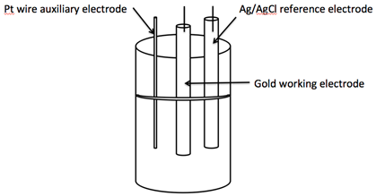Figure 1. A typical 3-cell electrode used in cyclic voltammetry

For the three-electrode electrochemical cell, the working electrode is a gold disk electrode. The auxiliary electrode is a platinum wire and the reference electrode is a silver-silver chloride electrode. In this type of cell the oxidation reaction occurs at the surface of the gold working electrode. The working electrode can act as either the anode or the cathode depending on the voltage being applied. The auxiliary electrode will then assume the role of the anode/cathode depending on what the working electrode is acting as[3]. The current flow is measure between the working and auxiliary electrode. The reference electrode has a constant known potential is used then to measure the potential where the redox reaction is taking place. Therefore the potential is measured between the working electrode and the reference electrode[4].

2.1. Chronocoulometry

Chronocoulometry is the measurement of charge per unit time[5]. In this technique the experiment starts at a potential where no reaction is occurring and stepped instantaneously to a potential where either the oxidation or reduction occurs. The charge measured during this step is then plotted in a charge vs. time^1/2 graph.

Once graphed we can then use the Cottrell equation:

(1)

Either of the steps of the graph will have a slope of 2nFACD^1/2π ^-1/2 where n, F, C, and D are the number of electrons transferred (in this case n=1) Faraday constant (in Coulombs/mole), concentration of analyte in solution (in moles/cm³) and diffusion constant of the analyte (in cm²/s^-1)[6]. From this data the surface area of the electrode can be determined.

2.2. Cyclic Voltammetry

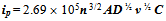
The general class of experiments in which the current from a working electrode is plotted versus the potential of the working electrode (relative to some reference electrode) is known as voltammetry. Cyclic voltammetry (or CV) is one of the most common forms of voltammetry and is routinely applied in labs today[7]. In cyclic voltammetry, the potential waveform applied to the working electrode is usually a triangle waveform. The potential is scanned back and forth linearly between two limits while the working electrode current is recorded. In a typical CV experiment, the solution is left static (meaning not stirred) during the recording of the cyclic voltammogram[8]. Under these static conditions the measured redox current is determined by several factors including the reactant concentration, electrode area, the diffusion coefficient and potential sweep rate. Here, we will discuss redox current observed on a disk electrode having relatively “large” surface area (> 100 μm in diameter). The equations described here cannot be applied for electrodes having very small sizes or different shapes[6].

In a static solution, there are several factors that need to be considered[9]. Since the electrode and solution are static, the species being oxidized or reduced at the electrode surface is depleted in the region nearest the electrode. As the potential is scanned past the redox potential of the species in solution, the current increases and then decreases as all the reactant is used up (at least near the electrode). For the potential sweep in the cathodic (or anodic) direction, the analyte is reduced (or oxidized) at the electrode. Upon sweep reversal, the reduced analyte is re-oxidized (or re-reduced). Hence, positive and negative current peaks are obtained, which are plotted as a cyclic voltammogram. If the electrode reaction is reversible, the peak current, i_p is given by:

(2)

where n is the stoichiometric number of electrons passed (e.g., n = 1 for Fe(CN)₆^3- + e- <=>Fe(CN)₆^4-), A the electrode area in cm², D the diffusion coefficient of the redox species in cm²/sec, v the scan rate in V/s, and C the concentration of the redox species in mol/cm^3[6]. Note that the origins of the current (i.e., from a reduction or oxidation) are not specified. Indeed, in a reversible system, i_pc and i_pa, the cathodic and anodic peak currents, should be almost identical. It can also be shown that in the reversible systems, the separation in potential for the anodic and cathodic peaks should be (for a diffusion-limited system):

(3)

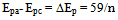
whereis in units of mV. For reversible redox processes, it is possible to obtain information on the “identity” of the redox species. The formal reduction potential, E^o’, can be found at the average of the two peak potentials[6, 10].

In this experiment you will be determining the area of the electrode, the formal reduction potassium ferricyanide, and the effects of varying concentration and scan rate.

3. Experimental

3.1. Solution Preparation

The instructor prepared 250 mL of 0.1 M KCl and a 100 mL stock solution of 10 mM K₃Fe(CN)₆ prepared in 0.1M KCl. The students prepared 25mL dilutions of the stock solution to 2.0, 4.0, 6.0 and 8.0 mM solutions.

3.2. Polishing the Electrodes

All three gold electrodes must be polished prior to use. This procedure serves the purpose of removing any contaminants from the electrode surface. To polish the electrodes, use a small amount of alumina on a polish cloth. Gently polish the electrode in a “figure 8” pattern for one minute. Then rinse the electrode with deionized water.

3.3. Reference and Auxiliary Electrodes

The reference electrode used in this experiment is a Ag/AgCl electrode. Do not leave the reference electrode sit in the ferricyanide solution for extended periods. When done with the reference electrode, rinse throughly with deionized water and store properly. The platinum auxiliary electrode should be rinsed with water prior to use.

4. Procedure

4.1. Determination of Surface Area of the Electrode

This first step is used to determine the area of the electrode. First the student will add the 2 mM K₃Fe(CN)₆ solution to the electrochemical cell. Insert the working, reference and auxiliary electrodes into the cell. Attach the green clip to the working electrode, the white to the reference and the red to the auxiliary electrode. Under “setup in the menu, select “Technique” and “Chronocoulometry”. Set the following parameters under “Parameters:” Initial Potential: 0.0V; Final Potential: 0.8V; Number of steps: 2; Sensitivity: 1e-6 A/V. Record a chronocoulometric plot for the solution. Repeat two more time for three trials total.

4.2. Running a Cyclic Voltammogram

This first step is to familiarize the student with the software and how to set up the experiment. First the student will add the 2 mM K₃Fe(CN)₆ solution to the electrochemical cell. Insert the working, reference and auxiliary electrodes into the cell. Attach the green clip to the working electrode, the white to the reference and the red to the auxiliary electrode. Set the following parameters: Initial Potential: 0.0 V; High Potential: 0.70 V; Low Potential: 0.0 V; Scan Rate: 0.20 V/s; Sweep Segments: 2; Sensitivity: 1e-6 A/V.

Record a cyclic voltammogram for the K₃Fe(CN)₆ solution. Adjust the sensitivity as needed. Repeat for the other two electrodes.

4.3. Effect of Scan Rate

Once the student is familiar with the software have them run the cyclic voltammetry experiment again using 2 mM K₃Fe(CN)₆ varying the scan rate between 0.025 V/s and 1 V/s. Adjust the sensitivity as needed and repeat for the other two electrodes.

4.4. Effect of Concentration

Once the student is familiar with the software have them run the cyclic voltammetry experiment again this time maintaining the scan rate at 0.20 V/s and using the K₃Fe(CN)₆ solutions between 2 and 10mM. Adjust the sensitivity as needed and repeat for the other two electrodes.

5. Results

To determine the area of the electrode a typical chronocoulometic plot is shown below in Figure 2.

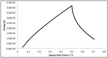Figure 2. Typical chronocoulometric plot for a 2 mm gold electrode in 2 mM K3Fe(CN)6 prepared in 0.1M KCl vs. Ag/AgCl

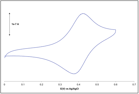Figure 3. Typical voltammogram plot for a 2 mm gold electrode in 2 mM K3Fe(CN)6 prepared in 0.1M KCl, 0.20 V/s vs. Ag/AgCl

From Equation 1 the student can calculate the area of the electrode given the diffusion constant of K₃Fe(CN)₆ is 7.6 x 10^-6 cm² s^-1 and the slope of the second step of the chronocoulometric plot. The student should discuss any differences in the experimentally calculated areas as well as what the area would be based on the area of a circle given a 2 mm diameter electrode.

From the cyclic voltammetry data the student should have a cyclic voltammogram as seen in Figure 3.

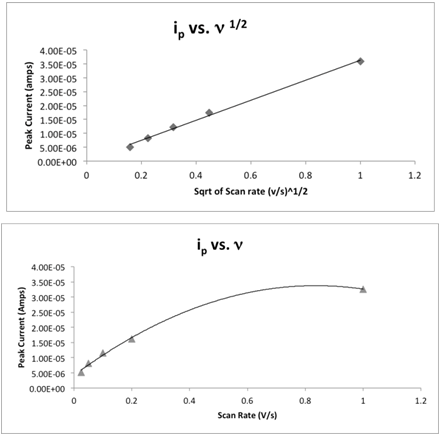Figure 4. Typical plots for (a) peak current versus scan rate and (b) peak current versus square rate of scan rate for a 2 mm gold electrode in 2 mM K3Fe(CN)6 prepared in 0.1M KCl vs. Ag/AgCl

The student should label the voltammogram with E_pc, E_pa, i_pc and i_pa. They should also calculate the formal reduction potential and and discuss any differences from literature values.

To demonstrate the effect of scan rate the student should provide a plot of 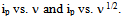Examples of these plots are shown in Figure 4. From the plot as well as Equation 2 the student should discuss which is the linear plot and why that is to be expected.

Finally to demonstrate the effect of concentration, the student should provide a Beer’s plot of i_p vs. concentration. The plot should be linear as shown in Figure 5. Depending on time constraints the laboratory instructor could provide a unknown concentration of K₃Fe(CN)₆ solution and the student uses the Beer’s plot to determine the concentration.

6. Conclusions

This lab has been shown to be very successful in demonstrating how electrochemical experiments are run as well as showing the kinds of information that can be obtained from these experiments.

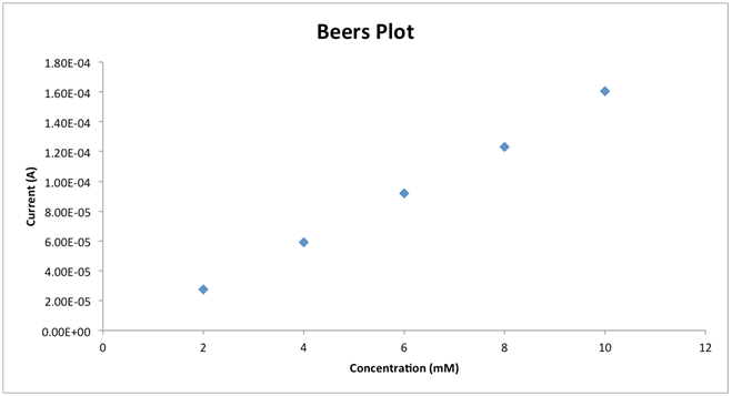Figure 5. Typical Beers plot for a 2 mm gold electrode in 2 mM K3Fe(CN)6 prepared in 0.1M KCl, 0.20 V/s vs. Ag/AgCl

ACKNOWLEDGEMENTS

The author wishes to thank the students in the Suroviec research lab as well as those students in Instrumental Analysis for helping to develop this lab. Thanks also to the Berry College Chemistry Department for providing financial resources