1. Introduction

One resumes the topic already dealt with in several articles: the “profitable close down”. One supposes that the products sold are substitutable. And the method used is Bertrand competition, with the demands deduced from the consumers’ utilities [1] [2]. A multivendor closes an asset, stopping the sales of a product, and makes a gain. This, because the competitor, a monoproduct firm, increases its price as a consequence of the retrieval of a rival product. It allows the multivendor to increase the price of the product it keeps selling, hence a gain which compensates and beyond the loss incurred due to the close down. The strategic effect allows a gain beyond the loss triggered by the direct effect.

Of course there is a condition. Even, the possibility of a “profitable close down” can be considered as a criterion: a criterion of saturated market. It remains that the term “saturated market” has to be interpreted. It is done in the conclusion.

The condition (of a “profitable close down”) is obvious. Let us call E₁ the monoproduct firm selling the product 1 and E the multivendor selling the products 2 and 3. The product 3 is retrieved from the market. P_i is the profit from the sales of the product i at the start (it is a Nash equilibrium, with E maximizing P₂ + P₃ given the choice of E₁ and E₁ maximizing P₁ given the choice of E). At the end, there is a Nash equilibrium with two products sold, 1 and 2, and the profits are P’_i. The condition is:

P’₂ > P₂ + P₃.

Of course, E decides the “close down” only if it allows a gain.

Concerning the prices there are two cases:

- The three prices increase. It is obvious that the consumers’ surplus decreases.

- One of the prices, that of the product “kept” (the product 2) can decrease [2]. One has to describe, in this case, the consequences of the “profitable close down”. It is the goal of this article.

It matters because the fall of a price can occur. Indeed, it should be small. One can deduce that from the declarations of the managers of large firms. In general, everything about the strategy of large firms is confidential. And the communication between the managers and the regulator is part of it. But often the managers appeal to the Opinion because it allows some pressure on the regulator. In these statements, the managers promise that there will be no increase of the prices. They do not dare to announce a decrease of prices (in case of mergers). Hence the pragmatic argument: a decrease of a price is possible (when a profitable “close down” occurs), but is should be small. In the paper, one chooses a condition concerning the prices: one of them can decrease a little. And a demonstration is needed to be certain that the consumers’ surplus decreases, in this case.

The model used is not the one which has been set out in the article “Evaluation of the monopoly as a stable second best” [2]. This model did not show the steps of the “close down”. The model used in this article shows the steps. It has been sketched in “Introducing a vision of regulation more complex than the traditional one” [3].

The plan of the article is:

- The model used is set out.

- Demonstration of the result.

- In the Conclusion, one comments on the regulator’s choices. He has to choose between two incommensurable options: affordability (the welfare of the consumers is taken into account) or financing innovation (the priority is high revenues for the firms, which will invest them in research on new products). It appears that the regulator is not an expert, but a strategist.

2. Methods and Results

2.1. Setting out the Model Used

To set out the model used, one starts by quoting a passage in the author’s article “Introducing a vision of regulation more complex that the traditional one” [3]:

- “p_i0 is “adapted” to p_j0 and p_k0 if: ∂ R_i / ∂ p_i (p_i0, p_j0, p_k0) = 0. That is to say, p_i0 is the best response of E_i, to p_j0 and p_k0.

- Let us call O p_i p_j [p_k = p_k0] the axes O p_i p_j if p_k = p_k0, with the reaction functions R_i and R_j (for p_k = p_k0). If p_i0 is “adapted” to p_j0 and p_k0, in O p_i p_j [p_k = p_k0] the point (p_i0, p_j0) is on R_i. Or, in O p_i p_k [p_j = p_j0] the point (p_i0, p_k0) is on R_i.

Suppose E₁ sells the product 1 and E sells the products 2 and 3. There is a Nash equilibrium (p₁₀, p₂₀, p₃₀). In O p₂ p₃ [p₁ = p₁₀], p₃ increases as far as p₃ = 1. The representative point moves vertically as far as p₃ = 1. The product 3 is no more sold (since one supposes D_i = 0 if p_i = 1).

One supposes a unique, stable Nash equilibrium when product 3 is no more sold.

In O p₂ p₃ [p₁ = p₁₀], the representative point moves on the line p₃ = 1 as far as the reaction function R₂ (p₂ = p’₂, p₃ = 1). When p₂ = p’₂, E is “adapted” to p₁ = p₁₀ and p₃ = 1. On O p₁ p₂ [p₃ = 1] the representative point (p₁₀, p’₂) is on R₂. In O p₂ p₃ [p₁ = p₁₀], the representative point went to R₂, sliding to the left or to the right:

- If p₂ increased (from p₂₀ to p’₂) the best response of E₁ is an increase (because p₂ increased and p₃ also). Therefore, on O p₁ p₂ [p₃ = 1], the representative point goes to the Nash equilibrium thanks to increases of p₁ and p₂. At the start, the point is on the lower strand of R₂. The prices p₁ and p₂ increase.

- If p₂ decreased, one does not know the best response of E₁ (to increase or to decrease its price), because p₂ decreased and p₃ increased. If the best response of E₁ is to increase p₁, the reasoning is the same than in the case dealt with. At least the price p₁ increases. The hypothesis of p₁ decreasing is impossible. The representative point would be on the higher strand of R₂. At the start, the profit P₂ is less than Max P₂ + P₃ (if p₁ = p₁₀). When the point slides alongside R₂ the profit P₂ decreases. Therefore, it cannot be more than Max P₂ + P₃ (if p₁ = p₁₀).

The three prices increase or at least two (the price of the product which is no longer sold and the price of the product of the competitor of the multiproduct firm).

If the three prices increase, the consumers’ surplus decreases. If two only increase, it is not sure”.

Therefore, one has to demonstrate that the consumers’ surplus decreases, when one of the prices (that of the product still sold by the multivendor) decreases. It is the goal of this article.

Representing the two first steps.

At the start, there is the point P, in O p₂ p₃ [p₁ = p₁₀]. One supposes symmetry of the consumers’ utilities, therefore of the demands: D₂ (p₁₀, p₂, p₃) = D₃ (p₁₀, p₃, p₂), for instance. There is the same for p₂₀ or p₃₀ fixed. Therefore, P is on the diagonal, where P₂ + P₃ is maximal. Its coordinates are (p₁, p₀, p₀), one calls the quantities D₂ (P) = D₃ (P), x, D₁ (P)= y. And in P, P₂ = P₃ = x p₀, P₁ = y p₁, the total profit is 2 x p₀ + y p₁.

During the first step, p₃ increases from p₀ to 1. The quantities become (y + Δ’, x + Δ, 0), with Δ > 0 and Δ’ > 0. The total quantity decreases, since the price p₃ increases: Δ + Δ’ – x < 0. The representative point slides as far as Q (see figure 1).

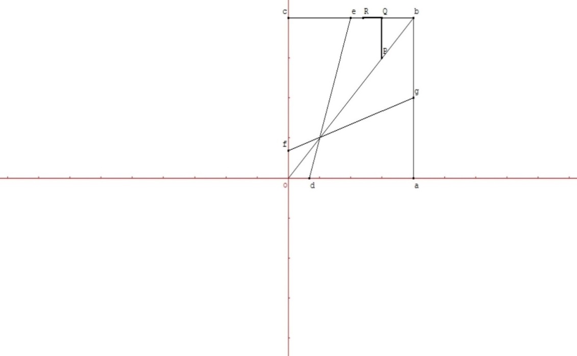Figure 1. The two first steps are represented by PQ and QR. de: R1. fg: R2. The coordinates are for P: (p1, p0, p0), for Q: (p1, p0, 1), for R: (p1, p’0, 1)

During the second step, the representative point, slides on p₃ = 1, as far as R (p₁, p_’0, 1). The price p₂ decreases from p₀ to p’₀ (p₁ < p’₀ < p₀). Here, the quantities are and . The price p’₀ corresponds to Nash equilibrium, N, with two products sold (1 and 2): N (p’₀, p’₀, 1).

Representing the two last steps.

It is in O p₁ p₂ [ p₃ = 1]. The second step QR is on the vertical with abscissa p₁. The price p₂ decreases from p₀ to p’₀. Then the third step is horizontal, from R to N (p’₀, p’₀). In N the quantities are D₁ = D₂ = x’, the profits are P₁ = P₂ = x’ p’₀. The total profit is 2 x’ p’₀.

Notice that the condition “profitable close down” is written: 2 x p₀ < x’ p’₀.

The two last steps are represented on Figure 2.

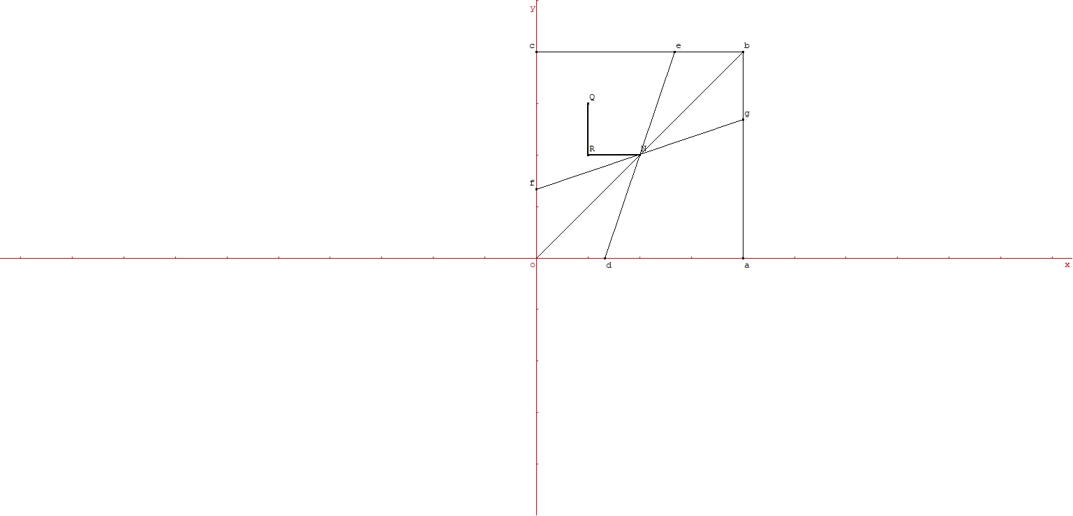Figure 2. The two last steps are represented by QR and RN. de: R1. fg: R2. The prices are, for Q: (p1, p0, 1), for R: (p1, p’0, 1), for N: (p’0, p’0, 1)

2.2. Demonstration of the Result

2.2.1. Study of a Certain Curve

Let us call region A the region limited by p₁ = 0, p₂ = 1, R₁, and p₁ = p’₀.

Also, one calls:

- region 1: Inside A, P₁ > P₂

- region 2: inside A, P₂ > P₁.

Region 1 and region 2 are separated by a continuous curve Г.

Imagine a point on the bisector, below N, going up along the vertical. At the start, P₁ = P₂, then the two increase as far as R₂. On R₂, either (1) P₁ > P₂, then P₁ increases and P₂ decreases, so there is no point where P₁ = P₂ (2) P₁ < P₂ and there is a single point where P₁ = P₂.

The curve Г, which passes by (0, 1) and N, is cut by a vertical in zero or one point.¹

Now imagine a point on p₁ = p’₀ above N. Here P₁ > P₂. If it slides along the horizontal line towards the left, as P₁ and P₂ decrease, and on p₁ = 0, P₁ = 0, P₁ < P₂, there is one point where P₁ = P₂, or an odd number of such points. Therefore, Г is cut by a horizontal line at least in one point, perhaps in several points.

The shape of the curve Г could be like in the figure 3, with a “hole” or several “holes”.

But it is impossible. One could pass from (0, p’₀) where P₂ > P₁ to (p’₀, 1) where P₁ > P₂ continuously, without any point where P₁ = P₂. Put in other words: the regions 1 and 2 are connected and there is a continuous frontier which separates them. Therefore, there are no “holes”.

The curve Г could be made up of several strands (separating the regions 1 and 2) and one or several arches of R₂.

One demonstrates a lemma.

Lemma. Alongside the curve Г from (0, 1) to N p₂ / p₁ always decreases.

The demonstration is easy and has been put in the Appendix 1.

A possible path can be described: from (0, 1) to N, one follows a strand of Г as far as R₂, then an arch of R₂ where P₁ > P₂ then possibly an arch or several of Г with arches of R₂ between them, p₂ / p₁ decreasing from to 1. It is obvious that on an arch of R₂ concerned, P₁ > P₂. Let us call x₁ and x₂ the ends of such an arch. Between the verticals passing by x₁ and x₂, and above R₂, there is no point where P₁ = P₂ since there is no point of Г. Therefore, in x₃ on the arch between x₁ and x₂, P₁ > P₂.

What matters for us is the shape of the curve above p₂ = p’₀. The shape is shown in the figure 3. There is a strand going down from (0, 1) to p₂ = p’₀ then, possibly one arch or several arches. Between the arches, there are segments of p₂ = p’₀.

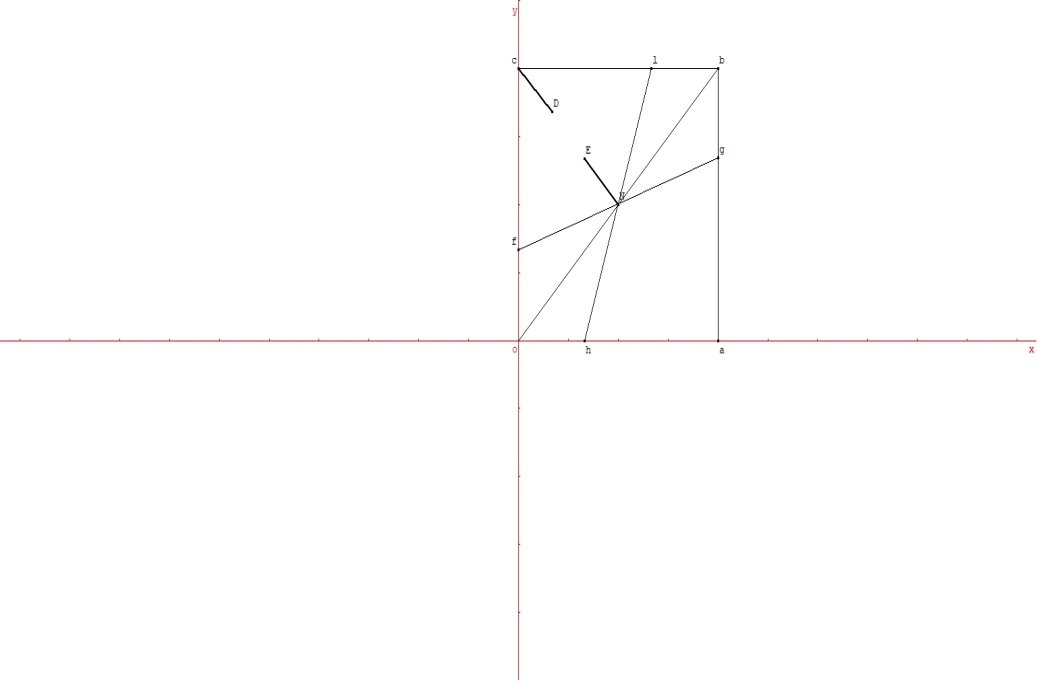Figure 3. The curve Г (c D E N) is shown. In this case, there is a “hole”. hl: R1. fg: R2

Also, the slope of Г at N is 1.

The slope of Г is – A / B with:

A = ∂ P₁ – P₂ / ∂ p₁ = D₁ + p₁ ∂ P₁ / ∂ p₁ – p2 ∂ D2 / ∂ p1

B = ∂ P₁ – P₂ / ∂ p₂ = p₁ ∂ D₁ / ∂ p₂ – D₂ – p₂ ∂ D₂ / ∂ p₂

In N, A = D₁ – p’₀ ∂ D₂ / ∂ p₁, B = p’₀ ∂ D₁ / ∂ p₂ – D₂, and D₁ = D₂, ∂ D₁ / ∂ p₂ = ∂ D₂ / ∂ p₁.

Therefore, at some point Г drops below p₂ = p’₀, to reach the bisector. Either Г is tangent to the bisector at N. The last part of Г is a curve between R₂ and the bisector, tangent to the bisector at N. Either the last part of Г is a segment on the bisector, an end of which is N.

A numerical example is set out in the Appendix 2. In this example, Г is made up of a strand, from (0, 1) to some point on the bisector, then a segment of the bisector, as far as N (see Figure 4).

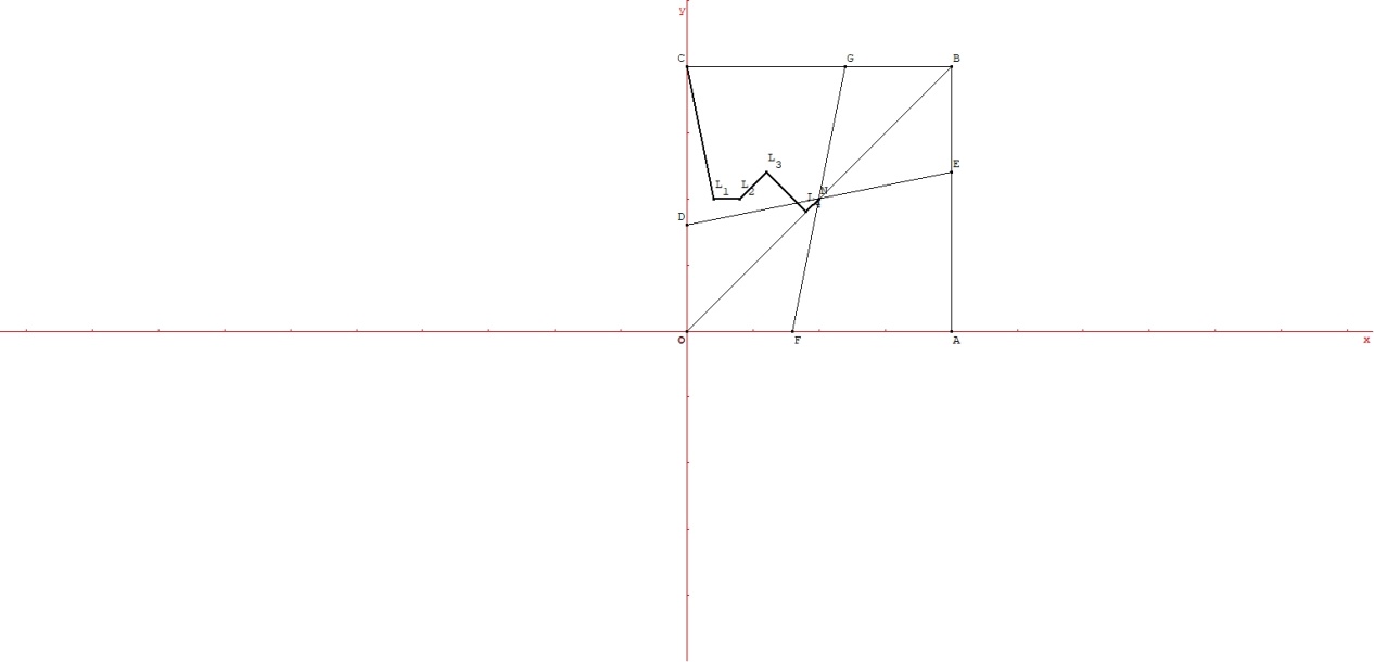Figure 4. An example of curve Г is shown: it is C L1 L2 L3 L4 N. First, there is a decreasing strand C L1, then a segment L1 L2 part of p2 = p’0, then an arch and the curve drops below p2 = p’0, reaches the bisector, the last part being a segment of the bisector, L4 N. DE: R2. FG: R1

But we are not done with the study of the curve Г.

Now we demonstrate an interesting lemma.

Lemma. Alongside Г, a point where p₁ p₂ is maximal is impossible.

One uses a proof by contradiction.

One supposes such a point, β. It is a point where the slope of Г is negative (at this point Г is tangent to the hyperbola (p₁ p₂ = Constant). Let us call H (Y) the hyperbola (p₁ p₂ = Constant) passing by the point Y, and CS (Y) the contour line for the function consumers’ surplus, passing by Y.

One considers a point α, above β, on Г, as near from β than one wants.

The curve Г is the locus of P₁ = P₂, separating the two regions, the region 1 where P₁ > P₂ and the region 2 where P₁ < P₂. In the region 1, at any point the slope of CS is lower than that of H. And in the region 2, at any point the slope of CS is higher than that of H.

The reader can easily check that:

- at α, where the tangent to CS and H has a lower slope than that of Г, H (α) “envelops” CS (α): the W strand of CS (α) is above H (α), the E strand of CS (α) is also above H (α). If Г is concave or convex at α, does not matter.

- At β, the W strand of CS (β) is above H (β), but the E strand of CS (β) is below H (β). It does not matter if at β, Г is concave, convex, or if it is an inflection point.

That is impossible. If one supposes continuity, the E strand of CS cannot pass from above to below H, the distance between α and β being arbitrarily small. The strands of CS and H cannot coincide, since they are the contour lines of two different functions.

The argument can be presented in another way. Suppose an observer linked to a mobile frame: when α slides toward β, the observer for which the tangent to H or CS is fixed (it is the axis of the abscissas), sees H (α) and CS (α) above the horizontal axis. The two curves are convex. The they are tangent to the horizontal axis at the origin of the axes. The two curves become distorted, but H (α) remains below CS (α). And all of a sudden, at β, the strand of CS which is on the right is below H. That is impossible.

2.2.2. Demonstration of the Result

First, the condition which is chosen. It is: p₀ p₁ < p’₀². In other words, the decrease of the price p₂ (that is to say p₀ – p’₀) is small enough, so p₀ p₁ < p’₀². One could have chosen p₁ + p₂ < 2 p’₀. In this case the demonstration is straightforward: the slope of the segment Q N is more than – 1, so the slope of the curves CS being less than – 1, the consumers’ surplus decreases along the segment Q N (from Q to N). But the condition chosen is more “general”: p₁ + p₂ < 2 p’₀⇒ p₀ p₁ < p’₀².

Consider H (N). It cuts p₂ = p0 on the right to Q. And H (N) does not cut Г, since in any point of Г the quantity p₁ p₂ is less than p’02. In fact, at N, the quantity p₁ p₂ is equal to p’₀², Г and H (N) are tangent, the slope of the tangent being – 1. H (N) is on the right to Г.

The path along which the consumers’ surplus decreases, from Q to N is obvious: Q → point of intersection of H (N) and p₂ = p₀ → H (N) → N. The curve H (N) is in the region 1 so the consumers’ surplus decreases when a point on H (N) moves to the right.

3. Conclusions

We have made three hypotheses:

- The demand functions (deduced from the customers’ utilities) are “regular” (twice continuously derivable). The curves (profits …) which are concerned are also “regular”. The response functions exist and are increasing.

- The utilities, therefore the demands are symmetrical.

- There is the condition p₀ p₁ < p’₀². The decrease of the price of the product “kept” is small enough, so this condition is fulfilled.

Given these hypotheses, the model which is presented is an “experience of thought”. But it stimulates the thought about the phenomenon “profitable close down”.

The regulator has to possible choices (1) He takes into account the consumers’ welfare, and, since it decreases if the “close down” occurs, he prohibits it and (2) He can favor the financing of innovation and let the “close down” occur. When the three prices increase, the total profit increases. It is easy to demonstrate. As the “close down” is supposed profitable, it is enough if the monovendor makes a gain. This is the case. The order of the steps does not matter. Therefore, suppose that p₃ (the price of the product no more sold), then p₂ (the price of the product “kept”) increase, first. The profit of the monovendor increases, because its price does not change, and the demand for its product increases. When p₁ increases, it is to reach the Nash equilibrium, and again the profit P₁ of the monovendor, increases.

One can suppose that the total profit increases also when the price p₂ of the product “kept” decreases just a little. So, more money can be invested in R and D, innovation and upgrading the products sold.

The two choices are incommensurable. The choice which is made depends on the outcome of the social play. There are what the French sociologist Tarde calls ‘logical duels [4]. Some are ended, other are ongoing.

Let us give examples of such “logical duels”:

- Net neutrality. This “logical duel” has ended. Affordability has been definitively chosen. The providers of standard Internet services (operators, CDNs, Content Distribution Networks, …) are competitors. To choose affordability is justified when networked services are concerned: the utility of a customer increases with the availability of the service for the other customers. It is preferable if a large quantity of services are sold, thanks to affordable prices.

- Medicaments. The spokespersons of Big Pharma praise the profits of the firms in the pharmaceutical sector: they allow more research on new treatments, or medicaments (bio drugs …). They disapprove the manufacturing and the sale of generic medicaments. From this point of view, if the prices are low because many differentiated products are available for the consumers, it is only a “windfall” for the consumers.

A well-known advocate of affordability is Christensen. After him, a real innovation involves a breakthrough, utility for the users, and an affordable price [5] [6]. He gives as examples the personal computer, and the mobile phone. One could add Net neutrality.

It appears that the regulator is not an expert, he is a strategist.

Indeed, the array of his choices is wider than just affordability / financing of innovation. For instance, if a firm is threatened to disappear or to be dismantled, it can be saved if a competitor buys it. But there is a risk: the bought firm is managed by a multivendor, and this has consequences on the investment. In France, recently, in the sector of the sale of furniture, the n° 2 was Conforama and the n° 3 was But. Conforama met great difficulties and was saved when But bought it. After the merger, the n° 2 is But and the n° 3 is Conforama [7]. Notice that the model presented by the author in the Journal of Game Theory [2] shows this: when an independent brand is bought then integrated in a multivendor, how this brand is managed changes.

Appendix 1

One demonstrates this lemma:

Lemma. Along Г, from (0, 1) to N, the quantity p₂ / p₁ decreases.

The lemma is not used in the demonstration of the result which is the goal of this article. But it helps to know the shape of the curve Г in a better way.

Let us call:

A = ∂ P₁ – P₂ / ∂ p₁ = D₁ + p₁ ∂ P₁ / ∂ p₁ – p₂ ∂ D₂ / ∂ p₁

B = ∂ P₁ – P₂ / ∂ p₂ = p₁ ∂ D₁ / ∂ p₂ – D₂ – p₂ ∂ D₂ / ∂ p₂. B > 0.

The quantity p₂ / p₁ cannot have an extremum on Г:

A d p₁ + B d p₂ = 0, and:

- p₂ d p₁ + p₁ d p₂, simultaneously, is impossible.

It is enough to demonstrate that: A p₁ + B p₂ = O is impossible.

This expression is written:

p₁ [D₁ + p₁ ∂ D₁ / ∂ p₁ – p₂ ∂ D₂ / ∂ p₁] + p₂ [p₁ ∂ D₁ / ∂ p₂ – D₂ – p₂ ∂ D₂ / ∂ p₂]

Given P₁ = P₂ on Г, and ∂ D₁ / ∂ p₂ = ∂ D₂ / ∂ p₁, this expression is: p₁² ∂ D₁ / ∂ p₁ – p₂² ∂ D₂ / ∂ p₂.

This expression is positive.

p₁ ∂ D₁ / ∂ p₁ > - D₁ ⇒ p₁² ∂ D₁ / ∂ p₁ > - p₁ D₁ = - P₁. A minorant is – P₁.

p₂ ∂ D₂ / ∂ p₂ < - D₂ ⇒ p₂² ∂ D₂ / ∂ p₂ < - p₂ D₂ = - P₂ ⇒ - p₂² ∂ D₂ / ∂ p₂ > P₂. A minorant is P₂.

A minorant of the expression is – P₁ + P₂ = 0. Therefore, the expression is positive.

Appendix 2

One presents a numerical example of curve Г. In this particular case, the consumers’ utilities are defined: d (p₁, p₂) = 1, there is a homogeneous density of utility.

We shall calculate the demands, the profits, the coordinates of the Nash equilibrium, the equation of Г and check the properties of the curve Г.

The demands D₁ (p₁, p₂) and D₂ (p₁, p₂) are easy to calculate, since they correspond to the area (u₁ – p₁ > u₂ – p₂ and u₁ – p₁ > 0 for D₁, and u₂ – p₂ > u₁ – p₁ and u₂- p₂ > 0, for D₂). Therefore:

D₁ = 1 / 2 – p₂² / 2 + p₂ – p₁

D₂ = 1 / 2 + p₂² / 2 – p₁ p₂ + p₁ – p₂

The profits are written:

P₁ = p₁ [1 / 2 – p₂² / 2 + p₂ – p₁]

P₂ = p₂ [1 / 2 + p₂² / 2 – p₁ p₂ + p₁ – p₂]

For the Nash equilibrium:

+ 1 = 0

∂ P₂ / ∂ p₂ = 1 / 2 + 3 p₂² / 2 – 2 p₁ p₂ + p₁ – 2 p₂ = 0.

The coordinates of N are (√2 – 1, √2 – 1) or (0, 41, 0, 41).

The curve R₂ has for equation ∂ P₂ / ∂ p₂ = 0, is increasing (positive slope) and goes from (0, 1 / 3) to N.

The curve R₁ has for equation ∂ P₁ / ∂ p₁ = 0, is increasing (positive slope) and goes from N to (1 / 2, 1). (See figure 5).

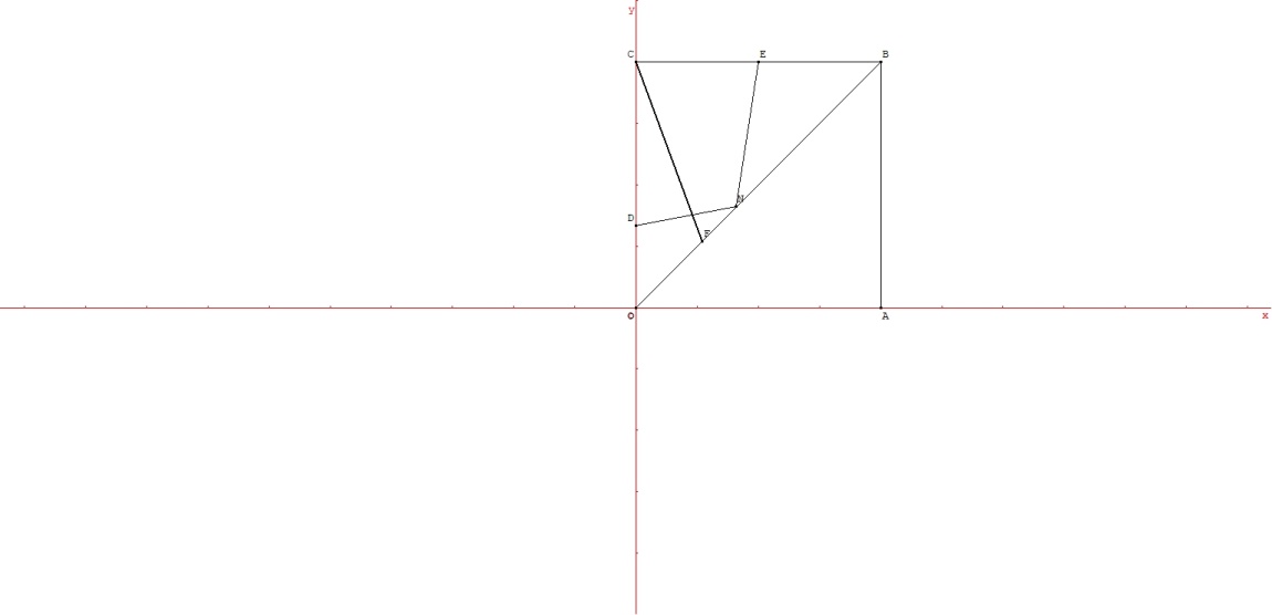Figure 5. The curve Г is shown: it is an arch of parabola going from C to F, then the bisector from F to N. The response function R2 is DN. The response function R1 is NE

The equation of Г is P₁ = P₂:

p₁ [1 / 2 – p₂² / 2 + p₂ – p₁] – p₂ [1 / 2 + p₂² / 2 – p₁ p₂ + p₁ – p₂].

Obviously, the equation holds if p₁ = p₂, therefore

(p₂ – p₁) is a factor:

(p₂ – p₁) [p₁ + p₂ – 1 / 2 – p₂² / 2] = 0.

Г is made up of two parts:

- An arch of parabola p₂² – 2 p₁ – 2 p₂ + 1 = 0. The summit is at (0, 1). The curve is decreasing, cutting the bisector at (0, 27, 0, 27), below N.

- The bisector from (0, 27, 0, 27) to N.

It remains to check this property of Г: p₁ p₂ reaches the value (√2 – 1)² only at N.

The equation of the parabola is (p₂ – 1)² / 2 = p₁ and one supposes that p₁ = (√2 – 1)²/ p₂. There is no root of this equation: (p₂ – 1)² / 2 = (√2 – 1)² / p₂.

The equation of the third degree:

p₂³ – 2 p₂² + p₂ – 2 (√2 – 1)² = 0 has no root between 0 and 1.

Note

1. In (0, 1) P₂ = 0 because one supposes D₂ (p₁, 1) = 0 for any p₁.