1. Introduction

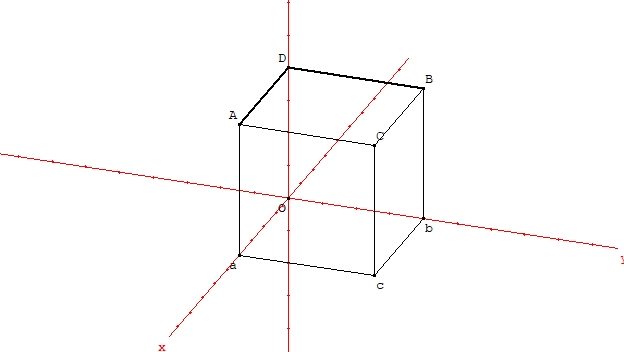
When one considers competitive equilibrium between differentiated products (Bertrand competition), it occurs that the Nash equilibrium is unstable. That is to say: a spontaneous process is possible, such that one product is withdrawn from the market. The concerned asset is bought then closed down, and the two operations are profitable [1]. A question is posed to the regulator, supposed to be unable to prohibit this process, which is detrimental to the consumers (the prices increase) [1]. This question is: what is the second best he should choose, the monopoly selling three products, or the Nash equilibrium after the withdrawal of a product (only two products are sold).

The article deals with this question.

One demonstrates in the article that there are three situations:

- The second best is the monopoly selling three products. Also, and it is a necessary condition, when the monopoly sells a new product, if generates more consumers’ surplus.

- The second best is the Nash equilibrium (two products being sold), but the monopoly selling a new product creates more consumers’ surplus.

- The second best is the Nash equilibrium (with two products sold) and the monopoly selling a new product does not create more consumers’ surplus.

A multiproduct monopoly has a strength and a weakness. The strength: it keeps the diversity of the products sold. It never cancels the sale of a product, its benefit would decrease. The weakness: it chooses high prices. So, the existence of two cases is explained. Either there is a real diversity of the products sold, and there is more consumers’ surplus created when the third product is sold (by the monopoly). Either it is a pseudo-diversity of the products sold, and the Nash equilibrium (only two products being sold) creates more consumers’ surplus than the monopoly (selling three products), because of the low prices. The second case is an intermediate one.

It is easy to provide examples of both.

It is also the opportunity to present the method used, Bertrand competition the demands being deduced from the consumers’ utilities. Here, in a frame Ou₁u₂u₃ (0 ≤ u_i ≤ 1) the density of utility is linear, homogeneous, equal to 1 / √2, on the bisectors of the faces of the cube u_i = 0 (figure 1). If it is the Nash equilibrium, the Bertrand paradox applies, and (with obvious notation): p₁ = p₂ = p₃ = 0, P₁ = P₂ = P₃ = 0. So, the player E₁ can buy and close E₃, then E_2, paying ε / 2 to each. Now the density is on O u₁, equal to 2/3, with a weight 1/3 at O. E₁ chooses p₁ = ½, its profit is 1/6 – ε, the consumers surplus is 1/12. If the regulator chooses the monopoly, the prices are p₁ = p₂ = p₃ = ½, and the consumers’ surplus is 1/8. Therefore, the monopoly is the second best. But, of course, the first best if the Nash equilibrium with three products sold, since the consumers’ surplus is ½. But it is unstable.

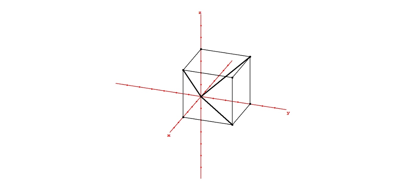Figure 1. The density of utility is linear homogeneous and on the bisectors of the faces ui = 0

Concerning an example of the second best being the Nash equilibrium (two products being sold), one can quote the example which is in the article of the author [1]. The density of utility is as on figure 2. The Nash equilibrium is unstable. The second best is obviously the Nash equilibrium. It creates a positive consumers’ surplus. The monopoly should choose p₁ = p₂ = p₃ = 1, and the consumers’ surplus would be 0. It is always the case, when the utilities are in the faces of the cube u_i = 1.

Figure 2. The density of utility is linear homogeneous on (0, 0, 1), (0, 1, 1) and (0, 0, 1), (1, 0, 1).

An interesting question is: does a monopoly selling a new product create more consumers’ surplus? The two are possible (it creates or not more consumers’ surplus). Here are two examples of both.

If the demands D₁, D₂, D₃ are independent, clearly the monopoly selling a new product creates more consumers’ surplus. For instance, the density is linear, homogeneous (equal to 1 / 3) and on the axes O u_i between 0 and 1 (figure 3). When the monopoly selling the products 1 and 2 sells the product 3, the consumers’ surplus increases from 1 / 12 to 1 / 8.

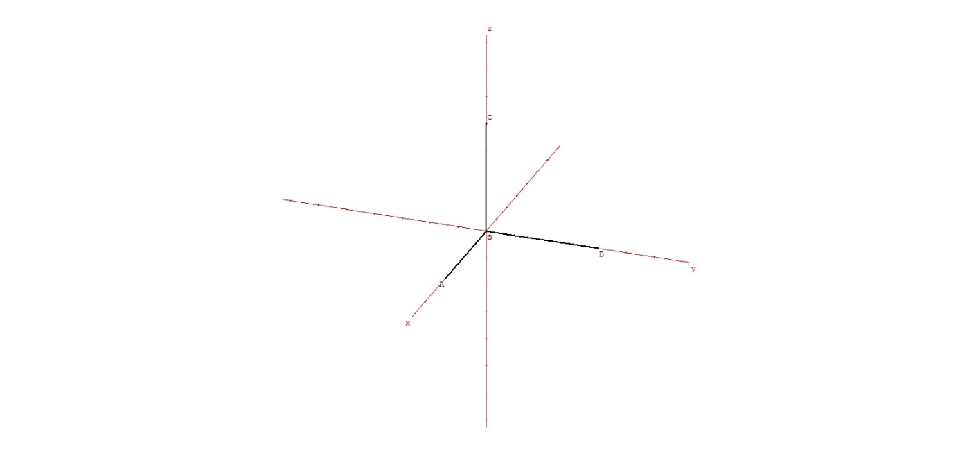Figure 3. The density of utility is linear, homogeneous on the axes O ui between 0 and 1

For an example of decreasing consumers’ surplus (when a monopoly sells a new product), consider this case: the density is areal, equal to 1 in the plane u₃ = 1 (figure 4). When the monopoly sells the products 1 and 2, the price is p₁ = p₂ = 0,57 (the calculation is made further in the paper). Therefore, the consumers’ surplus is positive. When the monopoly sells the product 3, also, it chooses p₁ = p₂ = p₃ = 1, and the consumers’ surplus is 0.

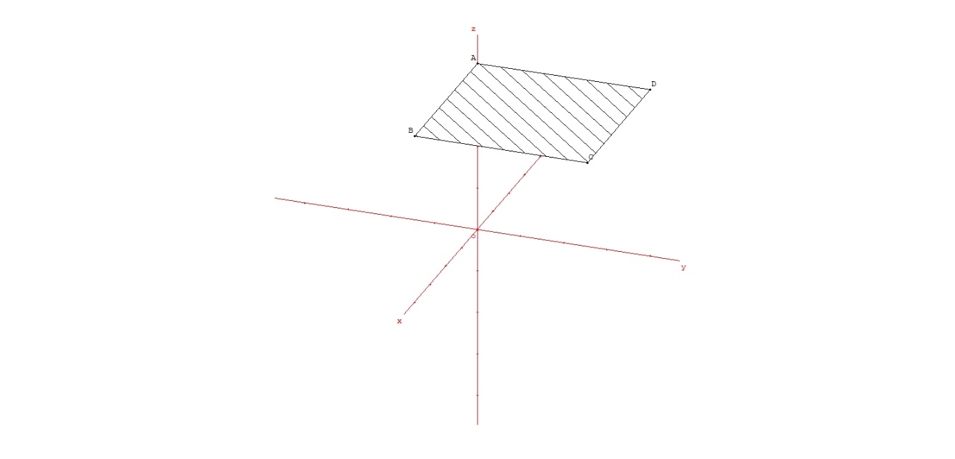Figure 4. The density is areal, homogeneous, equal to 1, in the plane u3 = 1

If one requires the Nash equilibrium being unstable, to have examples is easy, too.

In the tractable example which is described in the article, the Nash equilibrium is unstable and the monopoly selling a new product creates more consumers’ surplus.

For the other case (decreasing consumers’ surplus), one can resume the example quoted in the article of the author [2]. The utilities are in the faces of the cube u_i = 1. If the equilibrium is stable, non-differentiating innovation makes it unstable when pushed far enough [2]. And the monopoly selling the products 1 and 2 creates consumers’ surplus. When it sells the product 3, also, the consumers’ surplus is 0 (it chooses (p_0, p₀, p₀), the corner of the cube opposed to (0, 0, 0)).

Now, one can set out the plan of the article:

- Introduction

- The framework. The framework is presented. The main results are set out. The hurried reader could leapfrog the two successive chapters, then read the Conclusion.

- Results and demonstrations.

- A tractable, particular case is presented. It is the simplest case, with a density volumic, homogeneous, and equal to 1.

- Conclusion.

Some demonstrations, which are (a little) awkward, are put in Appendixes.

2. The Framework

In the frame O u₁ u₂ u₃ (0 ≤ u_i ≤ 1) there is a density of utility, the points (u₁, u₂, u₃) representing consumers with these gross utilities. For (p₁₀, p₂₀, p₃₀), D₁ (p₁₀, p₂₀, p₃₀), the demand for the product 1, is the quantity in the “pocket”:

u₁ – p₁₀ ≥ u₂ – p₂₀

u₁ – p₁₀ ≥ u₃ – p₃₀

u₁ – p₁₀ ≥ 0.

It corresponds to the consumers buying the product 1 because their net utility is maximized when they buy the product 1. It is obvious that D_i is decreasing in p_i, increasing in p_j and p_k. Also, if CS (p₁₀, p₂₀, p₃₀) is the consumers’ surplus, it is straightforward that d CS = -D₁ dp₁ -D₂ dp₂ – D₃dp₃, so (D₁, D₂, D₃) derives from a potential (-CS) and ∂D_i / ∂p_j = ∂D_j / ∂p_i. It is called Slutsky’s relation [3]. There are other interesting mathematical relations, such as ∂D₁ / ∂p₁ + ∂D₂ / ∂p₂ + ∂D₃ / ∂p₃ ≤ 0. Some will be used further in the article.

The functions D_i are supposed to be analytical, two times continuously derivable.

Concerning Bertrand competition, for p₃ fixed, one supposes a best response function R₁ (p₁, p₂) and R₂ (p₁, p₂): if the best response p₁₀ is obtained a single time (for p₂₀), R₁ is monotonic, and increasing because it is observed that the price increases from Nash equilibrium to monopoly (corresponding to p₂ = 1, that is to say D₂= 0). So, the prices are strategic complements.

One supposes a unique Nash equilibrium, therefore it is stable (in the sense that groping led the players to the equilibrium).

If the density is volumic, D_i = 0 if p_i = 1, for any p_j, p_k.

One supposes also a symmetry of the utilities about the planes u_i = u_j.

Now, one refers to figure 5.

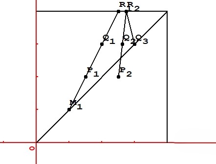Figure 5. The equilibrium points are shown on the bisector of the plane p3 = p30 when p30 varies from 0 to 1. Notice that the sign of the slopes of the curves is shown, but there are not necessarily straight lines

In coordinates, p₃ and in abscissas, it is the bisector of the plane p₃ = p₃₀, on which are the equilibrium points, given the symmetry (of the utilities):

- The points such as M₁ represent Nash equilibrium (for p₃ fixed). They are on the curve C₁: M_1, P₁, Q₁, R₁. The slope of C₁ is positive (in other words, the point representing Nash equilibrium slides toward the right when p₃ increases from 0 to 1). M₁, on the bisector p₁ = p₂ = p₃ represents the Nash equilibrium with three products.

- The points such as P₂ are the maxima of P₁ + P₂ (for p₃ fixed). They are on the curve C₂: P₂, Q₂, R₂. The slope is positive. The points representing the maxima of P₁ + P₂ slide toward the right, when p₃increases from 0 to 1. P₂ is the Nash equilibrium of E selling the products 1 and 2, and E₃ selling the product 3.

- The points like Q₃ are the maxima of P₁ + P₂ + P₃ (for p₃ fixed). They are on the curve C₃: Q₃, R₂ (the maxima of P₁ + P₂ and P₁ + P₂ + P₃ are the same when p₃ = 1 because D₃ = 0 and P₃ = 0 for p₃ = 1). The slope of C₃ is negative. Q₃ is the maximum of P₁ + P₂ + P₃ on the bisector p₁ = p₂ = p₃.

What is interesting is that the slope of C₃ is negative. The consequences are:

- If the monopoly selling three products is the second best (in Q₃) it is not thanks to price dominance (meaning that p’_i ≤ p_i for any i).

- If the second best is the monopoly (Q₃, not R₁), if the monopoly selling to products sells a new product, the consumers’ surplus increases. CS from R₁ to Q₃ is positive, Δ CS from R₂ to Q₃ is more, therefore it is positive. It is a necessary condition.

- If the Nash equilibrium is the second best (in R₁), Δ CS between R₁ and Q₃ is negative. Possibly, if the monopoly selling two products sells a new product, the consumers’ surplus increases (Δ CS is positive between R₂ and Q₃). It is the intermediate case. The tractable example below is thus. Possibly, when the monopoly selling two products sells a new product, it makes the consumers’ surplus decrease.

Therefore, the strength and the weakness of the monopoly appear. It keeps the diversity of the products sold, and it is favorable to the consumers. But choosing high prices is unfavorable to them. In case of a real diversity of the products, it creates more consumers’ surplus when it sells the product 3 and should be the second best. In case of pseudo-diversity of the products sold, when it sells the product 3, it makes the consumers’ surplus decrease. It is sure that the second best is the Nash equilibrium.

And there is the intermediate case: the products are differentiated, but not enough. The monopoly selling the product 3 makes the consumers surplus increase, but there are high prices, so the second best is the Nash equilibrium (with two products sold).

3. Results and Demonstrations

Several demonstrations are needed.

Proof that the curve C₂ is on the right of C₁.

The point of C₂ (choice of the monopoly selling the products 1 and 2, p₃ fixed) is such that ∂ P₁ + P₂ / ∂ p₁ = ∂ P₁ + P₂ / ∂ p₂ = O. Since ∂ P₁ / ∂ p₂ ≥ 0, ∂ P₁ / ∂ p₁ ≤ 0, the point is on the right of the point where ∂ P₁ / ∂ p₁ = 0 (on C₁).

Proof that C₃ is on the right of C₂.

A point of C₃ is such that ∂ P₁ + P₂ + P₃ / ∂ p₁ = ∂ P₁ + P₂ + P₃ / ∂ p₂ = 0 (p₃ fixed) so ∂ P₁ + P₂ / ∂ p₁ ≤ 0, since ∂ P₃ / ∂ p₁ ≥ 0. The point is on the right of the point where ∂ P₁ + P₂ / ∂ p₁ = 0 (on C₂).

Lemma.

When p₃ increases the unique point on the bisector, where ∂P₃ / ∂ p₃ = 0, moves to the right.

Oner writes: ∂ P₃ (p, p, p₃) = 0. One differentiates: 2 ∂² P₃ /∂ p₃ ∂ p₁ dp + ∂² P₃ / ∂ p₃² dp₃ = 0. The second term is negative (concavity of P₃ (p₁, p₂, p₃) for p₁ = p₂ = p, p₃ varying, and dp₃ ≥ 0). Therefore, dp ≥ 0 if ∂² P₃ /∂ p₃ ∂ p₁ ≥ 0. For p₂ = p fixed, consider the plane O p₁ p₃. The point where ∂ P₃ / ∂ p₃ = 0 is on the reaction function R₃, with a positive slope. Therefore

∂²P₃ /∂ p₃ ∂ p₁ ≥ O (one differentiates the equation of R₃ ∂ P₃ / ∂ p₃ = 0 in the plane O p₁ p₃).

A point such that ∂ P₃ / ∂ p₃ = 0 on the bisector (p₃ fixed), exists, because for any p₁ = p₂ fixed, when p₃ increases P₃ varies from 0 (p₃ = 0) to 0 (p₃ = 1). And this point is unique. The intersection of the surface ∂ P₃ / ∂ p₃ = 0 and the plane u₁ = u₂ is an increasing curve.

When p₃ starts increasing from 0, the point ∂ P₃ / ∂ p₃ = 0 meets C₁, first, in M₁, the Nash equilibrium with three products: ∂ P₁ / ∂ p₁ = ∂ P₂ / ∂ p₂ = ∂ P₃ / ∂ p₃ = 0. Then, p₃ increasing, it meets C₂ in P₂, representing the equilibrium of E selling the products 1 and 2, and E₃ selling the product 3: ∂ P₁ + P₂ / ∂ p₁ = ∂ P₁ + P₂ / ∂ p₂ = 0 and ∂ P₃ / ∂ p₃ = 0. Then, p₃ increasing, the point is on the right of Q₃, the choice of the monopoly selling three products, on the bisector p₁ = p₂ = p₃. Indeed, in Q₃, ∂ P₁ + P₂ + P₃ / ∂ p₃ = 0, therefore ∂ P₃ / ∂ p₃ ≤ 0 since ∂ P₁ + P₂ / ∂ p₃ ≥ 0.

Proof that the slope of C₁ is positive.

One differentiates ∂ P₁ / ∂ p₁ = 0 in p₁ and p₃: ∂² P₁ / ∂ p₁² dp₁ + ∂² P₁ / ∂ p₁ ∂p₃ dp₃ = 0. For dp₃ ≥ 0, dp₁ ≥ 0 because: ∂² P₁ / ∂ p₁² ≤ 0 (concavity of P₁ (p₁, p₃) in p₁ for p₂ fixed), and ∂² P₁ / ∂ p₁ ∂p₃ ≥ 0 (this is demonstrated considering the plane p₂ fixed, the axes O p₁ p₃, the point is on the reaction function R₁which has a positive slope).The curve of the reaction function R₁ is moving to the right, the curve R₂ is moving upward, the equilibrium point is moving on the right on the bisector p₁ = p₂.

The slope of C₁ is infinite at the point R₁. Indeed, ∂² P₁ / ∂ p₁ ∂p₃ is equal to 0 at this point.

∂² P₁ / ∂ p₁ ∂p₃ = ∂ D₁ / ∂ p₃ + p₁ ∂² D₁ / ∂ p₁ ∂ p₃. Also, ∂ D₁ / ∂ p₃ = ∂ D₃ / ∂ p_1. As D₃ (p₁, p₂, 1) = 0 for any p₁ and p₂, ∂ D₃ / ∂ p₁ = 0, ∂ D₁ / ∂ p₃ = 0 and ∂² D₁ / ∂ p₁ ∂ p₃ = ∂² D₃ / ∂ p₁² = 0.

Proof that the slope of C₂ is positive.

Indeed, the sign of the slope of C₂ is not known. It depends on the sign of ∂² P₁ + P₂ / ∂ p₁ ∂ p₃ (p, p, p₃). The sign of the slope is the same. One is sure that the slope is positive in R₂. It has been already demonstrated that ∂² P₁ / ∂ p₁ ∂ p₃ = 0 if p₃ = 1. And ∂² P₂ / ∂ p₁ ∂ p₃ = p₂ ∂² D₂ / ∂p₁ ∂p₃ is positive. In general, ∂² D_i / ∂p_j ∂p_k is positive. It is easily demonstrated. It is a consequence of the definition of the demands (the “pockets”).

If one supposes the curve C₂ monotonic, it is increasing. It is to add a hypothesis. In any way the sign of the slope of C₂ does not matter very much, given the purpose of the article (what matters is the sign of the slope of C₃).

The sign of the slope of C₂ at P₂ is uncertain.

What is demonstrated in the article of the author [1] is this: when the close down is profitable, with obvious notation, p_independent increases as far as a common value with p_kept while p_closed increases as far as 1. If the common value is reached with p_kept increasing, R₁ is on the right of P₂. It is obvious if P₂ is above the bisector (p₃ ≥ p₁). But P₂ is below the bisector (as it is represented on the figure 5). At P₂, ∂ P₃ / ∂ p₃ = 0 and ∂ P₁ / ∂ p₁ ≤ 0. In a plane p₂ fixed, in the axes O p₁ p₃, P₂ is on the reaction function R₃, with ∂ P₁ / ∂ p₁ ≤ 0, it is on the strand NE of R₃ and p₁ ≥ p₃. One does not know if R₁ is on the left or on the right of P₂. If it is on the right, the curve C₂ (supposed monotonic) is increasing, because R₂ is on the right of R₁. And the close down makes the consumers’ surplus decrease (the points P₂ and R₁ do not describe the close down, but the consumers’ surplus at P₂ and R₁ are the consumers’ surpluses before and after the close down).

The point R₁ could be on the left of P₂.

If the point R₁ is on the left of P₂, given that the slope of C₂ is positive at R₂, the curve C₂ (supposed monotonic) is increasing.

Proof that the slope of C3 is negative.

The demonstration is awkward and is put in Appendix 1.

4. A Tractable, Particular Case

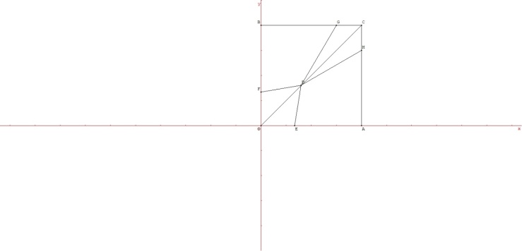
In this example, the density of utility is homogeneous, equal to 1.

The formulas giving the demands depend on the values of p₁, p₂, p₃. There are regions in a plane p₃ fixed (see figure 6). For instance, a region is: p₂ ≤ p₁ ≤ p₃.

Figure 6. The six regions in the plane O p1 p2 with 0 ≤ pi≤ 1 when p3 = 1 / 2. The hatched region corresponds to p2 ≤ p1 ≤ p3

In these conditions, the formulas of the demands are:

D₁ = p₃³ / 6 – p₂ p₃² / 2 + p₁² / 2 – p₃² / 2 – p₁ p₂ + p₂ p₃ – p₁ + p₂ / 2 + p₃ / 2 + 1 / 3.

D₂ = p₃³ / 6 – p₁ p₃² / 2 – p₃² / 2 – p₁² / 2 + p₁ p₃ + p₃ / 2 – p₂ + p₁ / 2 + 1 / 3.

D₃ = (1 – p₃) [1 / 3 + p₁ + p₂ / 2 + p₁ p₂ – (2 / 3 + p₁ + p₂ / 2) p₃ + p₃³ / 3].

To have the formulas in the other regions, one switches the indexes.

Now one finds the four equilibrium points N (Nash equilibrium with three products), N’ (Nash equilibrium with two products), P (monopoly selling three products), and P’ (monopoly selling two products).

Nash equilibrium with three products (N).

One uses the formulas above. One finds p₀ ≈ 0,32. The joint profit is P_N ≈ 0,31.

Monopoly selling three products (P).

One finds p₀ ≈ 0,63. The joint profit is P_P ≈ 0,47.

If p₃ = 1, one considers in axes O u₁ u₂ the areal density equal to 1 (figure 7). The calculations have been already presented by the author [4]. One can find the demands D₁ and D₂, making p₃ = 1 in the formulas above.

Figure 7. The density is areal and equal to 1. The demand D1 is shown for p1 = 1 /2 and p2 = 1 / 4

One finds p_N’ ≈ 0,41 and the joint profit is P_N’ ≈ 0,36.

Monopoly selling two products (P’).

One finds p₀ ≈ 0, 57 and the joint profit is P_P’ ≈ 0,47.

The four points are in the order described in the model. One has from the left to the right: N (0,32, 0,32, 0,32), N’ (0,36, 0,36, 1), P’ (0,57, 0,57, 1), P (0,63, 0,63, 0,63).

The equilibrium is unstable. The joint profit for the Nash equilibrium with three products (0,31) is less than the joint profit with two products (0,36). But the buy and close down is not profitable: 2 / 3 of P_N, (0,20), is more than 1 / 2 of P_N’, (0,18). Therefore, all what can happen is the withdrawal of a product thanks to lateral payments. But it is difficult [1]. It remains that the regulator can examine the question of the second best.

What is the second best?

It is the Nash equilibrium with two products.

As the demands derive from a potential, any path can be used to calculate Δ CS, the variation of the consumers’ surplus between two points. One chooses the path: N’ → (1, 1, 1) → P.

One has to calculate:

Δ CS = - ∫ (1 – p²) dp _{N’ → (1, 1, 1)} + ∫ (1 – p³) dp _{(1, 1, 1) → P.}

Δ CS = [p – p³ / 3]¹_0,41 + [p – p⁴ / 4]¹_0,63.

Δ CS ≈ - 0,12.

Another interesting question is: does the monopoly selling two products create consumers’ surplus when it sells a product more?

The answer is yes.

One has to calculate:

Δ CS = -∫ (1 – p²) dp _{P’ → (1, 1, 1)} + ∫ (1 – p³) dp _{(1, 1, 1) → P}

Δ CS = [p – p³ / 3] ¹_0,57 + [p – p⁴ / 4]¹_0,63

The quantity Δ CS is very small but positive: Δ CS ≈ 0,006.

So, the studied example corresponds to the intermediate case described above. The second best is the Nash equilibrium with two products. The monopoly selling two products creates consumers’ surplus when it sells a new product. In other words: the diversity of the products sold is real, but it is not enough to have the monopoly being the second best.

One has also to demonstrate that the tractable example has the characteristics of the model: the prices are strategic complements. As the demonstration is a little awkward, it has been put in the Appendix 2.

5. Conclusions

Interaction is not a catchword. It is a complex phenomenon, which deserves an accurate modelling. In this article the chosen model is Bertrand competition, the demands being deduced from the consumers’ utilities. One has made several hypotheses: (1) the reaction functions exist and are increasing (2) symmetry of the consumers’ utilities about the three planes u_i = u_j (3) unicity of the equilibria. In these conditions, it is difficult to state that one affords an accurate twin of the reality. Rather, an “experience of thought” is proposed. That game theory allows “experiences of thought” is set out by Ariel Rubinstein, a specialist of game theory [5]. A game theory model makes ponder: effects are isolated, studied and the model says how they add to give a kind of result. But it is an artefact, useful to allow reasonings.

An example is the “experience of thought” proposed in this article.

A multiproduct monopoly has a strength and a weakness:

- The strength is that it keeps the diversity of the products sold. A monopoly sells a new product as soon as it can, since it makes more profit. And it never closes down an asset (cancelling the sale of a kind of product). It is easily explained. One compares a multiproduct monopoly and a multiproduct firm with a competitor. The multiproduct firm with a competitor can possibly close down an asset, making a profit, because … it has a competitor. When the asset is closed down, the competitor increases its price (it is the strategic effect) and then, the firm which sells only one product, now, makes a gain. And it chooses a new price to optimize its profit. The strategic effect compensates and besides the loss due to the closing down (direct effect). It cannot occur if a multiproduct monopoly is concerned.

- The weakness is high prices. The multiproduct monopoly does not fear the stealing of market shares: in case of stealing of a market share, there is a gain compensating the loss, since the product the market share of which increases, is also owned by the multiproduct monopoly.

Finally, as one or the other of the two opposite effects is stronger, one has the three situations already described:

- The second best is the monopoly (selling three products). The diversity of the products sold matters. Also, if the multiproduct monopoly selling two products sells a new product, the consumers’ surplus increases. In some way, this is a criterium for a real diversity (differentiation of the products sold): when the monopoly sells a new product, selling three products, the consumers’ surplus increases.

- There is an intermediate situation. The diversity of the products sold is real (when the monopoly sells a new product, the consumers” surplus increases), but it is not enough. The prices are high. The Nash equilibrium (with two products) creates more consumers’ surplus.

- The second best is the Nash equilibrium (with two products). There is not a real diversity of the products sold. When the monopoly sells a new product, it does not create more consumers’ surplus.

So, two interesting criteria have appeared:

- A criterium for the Nash equilibrium (with three products) stable. It is: the entry of the third product increases the joint profit [1].

- A criterium for the diversity (differentiation of the products sold). It is: when the multiproduct monopoly sells a new product, the consumers’ surplus increases.

Notice that when the second best is the monopoly (selling three products) the close down triggers a decrease of the consumers ‘surplus. It is easily demonstrated, considering the consumers’ surplus during a chain of operations: P₂ → R₁ → Q₃ → P₂. This has a meaning for the regulator. Suppose he is coping with a product possibly withdrawn from the market (because the close down is profitable). If he must keep the diversity of the products sold (because the second best is the monopoly selling three products), there is a sign for him: the close down makes decrease the consumers’ surplus.

Of course, empirical studies are needed to check the validity of these criteria. For instance, such a study is the article quoted in the author’s article [1]. It is “Antitrust and innovation: welcoming and protecting disruption” [6]. So, the experience of thought allows reasonings and explanations, and also provides questions. Empirical studies complete the experience of thought, if they deal with the questions which are arisen by the experience of thought. In particular, it would be interesting to empirically study this question: does a multiproduct monopoly selling a new product, creates more consumers’ surplus?

We live in a “liquid society” [7]. All our choices are transitory and liquid: the city where we live, the job, the consumers’ s tastes etc. The assets are also liquid. Not only in the financial sense: an asset is liquid when it can be sold immediately, for a sum of money. But in this sense: an asset is deliberately close down, without any reason of bankruptcy. The author has already commented some cases [8]. The management of multiproduct firms can be very complex. In a portfolio of brands, there can be … thousands of brands [9]. Suppose a multiproduct firm closing down an asset. It is because it drives the prices down. The competitors outside the multiproduct firm, will increase their prices. It remains a competitor, inside the multiproduct firm, after the closing down. It benefits from the increase of prices (of the competitors outside the multiproduct firm). And the loss (due to the close down) is compensated and besides, by the gain.

There are two possible reasons when an asset can be closed down, and it is profitable: (1) the product generates a small utility, so the seller chooses low prices, to succeed in sales (2) the product is weakly differentiated from another product sold. This triggers a price war.

Appendix 1

Proof that the slope of the curve C₃ is negative.

One starts demonstrating that if p₃ = 1, ∂² P₁ + P₂ + P₃ / ∂ p₁ ∂ p₃ is negative.

The quantity ∂² P₁ + P₂ + P₃ / ∂ p₁ ∂p₃ can be written (at the point (p, p, 1):

∂ D₁ / ∂ p₃ + ∂ D₃ / ∂ p₁ + p [∂² D₁ + D₂ + D₃ / ∂ p₁ ∂ p₃] + (1 – p) ∂² D₃ / ∂ p₁ ∂ p₃.

∂ D₁ / ∂ p₃ = ∂ D₃ / ∂ p₁ is equal to 0 (D₃ = 0 if p₃ = 1).

The quantity between brackets is negative. It is a consequence of the definition of the demands (the “pockets”).

And ∂² D₃ / ∂ p₁ ∂ p₃ is negative if p₃ = 1.

If p₃ = 1, ∂ D₃ / ∂ p₁ d p₁ = 0 (with d p₁ ≥ 0).

If p₃ is just a little below 1 (d p₃ ≤ 0):

∂ D₃ / ∂ p₁ d p₁ > 0.

Therefore, ∂² D₃ / ∂ p₁ ∂ p₃ is negative.

Then one demonstrates that in Q₃, ∂² P₁ + P₂ + P₃ / ∂ p₁ ∂ p₃ ≤ O.

In Q₃ there is the unique maximum of P₁ + P₂ + P₃. Given the symmetry one has:

∂² P₁ + P₂ + P₃ / ∂ p_i² = a and ∂² P₁ + P₂ + P₃ / ∂ p_i ∂ p_j = b.

The Hessian matrix has for coefficients a_ii = a and a_ij = b. An obvious eigen value is b – a.

Therefore b – a ≤ 0 and a being negative, b ≤ 0.

The slope of C₃ in Q₃ and R₂ is negative.

One has to make one of these hypotheses:

- C₃ is monotonic

- C₃ is on one side, left of right, of the vertical passing by Q₃.

- Considering the vertical passing by Q₃, the value of ∂² P₁ + P₂ + P₃ / ∂ p₁ ∂p₃ is negative when p₃ = 1 and in Q₃. Suppose that this value is negative at any point of the segment. R₂ cannot be on the right side of the vertical. C₃ should cross the vertical, starting to the left from Q₃, then reaching the point R₂. And at the point of intersection, the slope should be positive. But this is impossible.

Accepting one of these hypotheses, the consequence is that the strand of C₃ is on the left side of the vertical. And R₂ is on the left of Q₃.

Appendix 2

One wants to prove that the curve R₁ (p₃ fixed), in the plane O p₁ p₂, is increasing. One studies the SE strand. At the start, when p₃ = 1, it is easy to prove it. The prices are strategic complements (figure 8).

Figure 8. The reaction functions R1 and R2 when p3 = 1 are shown. The shape is not linear. The strand SE, which is studied, goes from (1/3, 0) to (0,41, 0,41)

There is a discontinuity of the slope on the bisector, at the point which is the Nash equilibrium (0,41, 0,41). One has to prove that when p₃ decreases, the curves R₁ (p₃) remain increasing.

The strand SW is symmetrical (about the bisector). One needs also to study strand NE, the strand NW being symmetrical (about the bisector).

To study strand SE, one uses the formulas already set out (the case p₂ ≤ p₁ ≤ p₃).

The demonstration is awkward and needs several steps.

Step 1.

Lemma. The curve R₁ (p₃) cuts the bisector at a unique point (p₀, p₀), p₀ decreasing when p₃ decreases.

The formula for R₁ (p₃) is:

∂ P₁ / ∂ p₁ (p₁, p₂, p₃) = p₃³ / 6 – p₂ p₃² / 2 + 3 / 2 p₁² – p₃² / 2 – 2 p₁ p₂ + p₂ p₃ – 2 p₁ + p₂ / 2 + p₃ / 2 + 1 / 3.

Or:

∂ P₁ / ∂ p₁ (p₁, p₂, p₃) = A (p₁, p₃) + p₂ B (p₁, p₃)

A (p₁, p₃) = p₃³ / 6 + 3 / 2 p₁² – p₃² / 2 – 2 p₁ + p₃ / 2 + 1 / 3.

B (p₁, p₃) = - p₃² / 2 – 2 p₁ + p₃ + 1 / 2.

To find the intersection point of R₁ and the bisector one writes: p₁ = p₂ = p_0.

∂ P₁ / ∂ p₁ (p₀, p₀, p₃) = p₃³ / 6 +3 / 2 p₀² – p₃² / 2 – 2 p₀ + p₃ / 2 + 1 / 3 + p₀ (- p₃² / 2 – 2 p₀ + p₃ + 1 / 2).

One demonstrates that these is a unique root p₀, 0 ≤ p₀ ≤ 1, for p₃ fixed.

Also:

∂² P₁ / ∂ p₁ ∂ p₀ = - p₀ – 1 / 2 (p₃ – 1)² – 1, negative

∂² P₁ / ∂ p₁ ∂ p₃ = 1 / 2 (p₃ – 1)² + p₀ (1 – p₃), positive.

Therefore, when dp₃ ≤ 0, d p₀ ≤ 0. When p₃ decreases from 1, the intersection point moves towards the left. At some time p₃ “catches up” with p₀, p₃ = p₀ = 0,32. It corresponds to the Nash equilibrium with three products. The used formulas (p₂ ≤ p₁ ≤ p3) are no longer valid. But it does not matter because the equilibrium points which are calculated correspond to p₃ > 0,32.

Step 2.

Lemma. When p₃ decreases from 1 to 0,32, B remains positive.

B decreases from 0,18 (when p₃ = 1) to 0,13 (when p₃ = 0,32).

To prove that B decreases:

d B = - 2 d p₀ + (1 – p₃) d p₃

∂² P₁ / ∂ p₁ ∂ p₀ d p₀ + ∂² P₁ / ∂ p₁ ∂ p₃ d p₃ = 0.

d B is of the same sign than a quantity which is negative.

Therefore, B = ∂² P₁ / ∂ p₁ ∂ p₂ is positive.

And: ∂² P₁ / ∂ p₁² = 3 p₁ – 2 – 2 p₂, ∂² P₁ / ∂ p₁² (p₀, p₀, p₃) = p₀ – 2 ≤ 0.

The slope of R₁ (on the bisector) - ∂² P₁ / ∂ p₁² /∂² P₁ / ∂ p₁ ∂ p₂ is positive.

The slope of R₁ at the intersection with the bisector, is positive.

The curve R₁ passes below the bisector, since R₁ reaches p₂ = 0 without cutting the bisector, since there is a unique root of the equation ∂ P₁ / ∂ p₁ (p₀, p₀, p₃) = 0.

The strand of R₁ is entirely in the triangle ((0, 0), (p₀, p₀), (p₀, 0)). Indeed, p₂ = - A (p₁, p₃) / B (p₁, p₃), for p₁ = p₀ shows that there is a unique point of R₁ on the vertical passing by (p₀, p₀). This point is (p₀, p₀).

Step 3.

The curve R₁ is monotonic.

It is impossible that:

∂ P₁ / ∂ p₁ (p₁, p₂, p₃) = 0, and

∂ P₁ / ∂ p₁ (p’₁, p₂, p₃) = 0, with p₁ and p’₁ different.

One subtracts. A necessary condition is:

3 / 2 (p₁ + p’₁) – 2 – 2 p₂ = 0.

This is impossible. Since R₁ is in the triangle ((0, 0), (p₀, p₀), (p₀, 0)), p₁ ≤ p₀, p₂ ≤ p₀, and p₀ ≤ 0,41.

A majorant is 3 x 0,41 – 2 – 2 p₂ < 0.

This quantity is negative, not equal to 0.

The strand starts from p₂ = 0, is increasing as far as the point on the bisector (p₀, p₀).

The prices are strategic complements.

The strand slides toward the left when p₃ decreases (from p₃ = 1 to p₃ = 0,32).

Indeed:

∂² P₁ / ∂ p₁² = 3 p₁ – 2 p₂ – 2 < 0 (one has a majorant which is negative, replacing p₁ by 0,41).

∂² P₁ / ∂ p₁ ∂ p₃ = 1 / 2 (p₃ – 1)² + p₂ (1 – p₃) > O.

The strand slides starting from (1 / 3, 0) to (0,41, 0,41) when p₃ = 1, to (0,27, 0) to (0,32, 0,32) when p₃ = 0,32.