1. Introduction

The resolution of intricate problems frequently involves the amalgamation of diverse mathematical frameworks and computational methods. In the domains of differential games and bioeconomic models, characterized by complex interactions and dynamic systems, the accuracy and computational efficiency of numerical methods are crucial. This imperative has catalyzed the investigation into novel computational strategies, including the application of the Jacobi Tau method (JTM) approach, which has shown promise in tackling differential equations that are nonlinear and subject to complex constraints.

Differential game theory expands upon optimal control theory to examine the strategic interplay among several agents, each aiming to optimize their outcomes in the face of mutual competition. Recognized for its substantial influence in management sciences and economics, differential game theory’s applications permeate through various sectors, including resource management and the economics of ecosystems, as highlighted in foundational literature [1]. These applications range from marketing strategies to environmental economics and are further exemplified in studies on competitive dynamics in advertising [2] and the exploration of cooperative strategies within stochastic frameworks [3].

Central to the study of differential games are equilibrium concepts. The Nash equilibrium serves as a cornerstone in concurrent games, where individual strategy adjustments cannot enhance outcomes [4]. Differential games, however, introduce a nuanced classification: closed-loop versus open-loop equilibria. Strategies in the former are contingent on both temporal and state variables, while in the latter, they depend solely on time and initial conditions. Identifying optimal strategies within such games requires solving a system of equations rooted in fundamental game theory principles, which delineate the optimal response strategies among players [5]. Various analytical and numerical methods are employed to find solutions to these equations [6].

Given the limited availability of analytical solutions, numerical methods are indispensable for grappling with the complexities inherent in differential games. This area has been explored in depth, with studies ranging from linear quadratic dynamics ([7]-[11]) to nonlinear games addressing environmental concerns [12]. Certain scenarios, such as state-dependent scenarios [13] and zero-sum game frameworks [14], have further refined our understanding of equilibrium in differential games.

Among various numerical techniques, spectral methods have been lauded for their precision and efficiency, leveraging orthogonal polynomial series to resolve differential equations ([15]-[19]). These methods, applied within the context of Pontryagin’s maximum principle, are particularly potent for differential games, with the choice of method being influenced by the nature of the differential game in question [20,21]. This research introduces a pioneering numerical scheme that synergizes Pontryagin’s maximum principle with the JTM approach to ascertain the (OLNE) in noncooperative, nonzero-sum differential games.

In the confluence of mathematical theories, game theory, and computational analysis, the Jacobi Tau method approach emerges as a formidable tool, facilitating the transition from theoretical constructs to tangible, practical outcomes. This study ventures through the complexities of bioeconomic modeling and differential games, showcasing the potential of JTM to decode and address real-world economic and strategic challenges.

The study employs the Jacobi Tau Method (JTM) in synergy with Pontryagin’s Maximum Principle to solve the OLNE in noncooperative nonzero-sum differential games. This approach illustrates the potential of JTM in addressing complex bioeconomic modeling and differential games, highlighting its capacity to handle real-world economic and strategic challenges.

In summary, optimizing bioeconomic models involves a delicate balance of ecological sustainability, economic viability, and social acceptability. It requires an interdisciplinary approach that combines insights from biology, economics, mathematics, and social sciences. Advanced computational methods, like the Jacobi Tau Method, play a crucial role in addressing these challenges by providing more accurate and efficient tools for modeling and solving complex bioeconomic problems. In the realm of differential games and bioeconomic modeling, the Jacobi-Tau Method (JTM) stands out for its remarkable accuracy and computational efficiency, particularly when addressing complex interactions and dynamic systems. This method, developed to handle nonlinear differential equations and intricate constraints, shows a clear advantage over other methods like the Legendre Tau method. While the Legendre Tau method has been effective in solving open-loop Nash equilibrium problems in noncooperative games, the JTM's capability to handle more complex dynamics and constraints suggests a significant advancement in applied mathematics and engineering. Its potential in revolutionizing numerical analysis and enhancing simulation methodologies marks it as a promising tool for further research and applications in differential games and bioeconomic modeling, outperforming existing methods in key aspects.

2. Problem Statement

In this segment, we address the dynamics of a four-player differential game characterized by noncooperative interactions and non-zero-sum payoffs as delineated below:

2.1. Definition

We characterize a noncooperative nonzero-sum four-player differential game in the following manner [22]:

subject to

(1)

where are indices that belong to the set {1, 2, 3, 4}, each one distinct from the others.

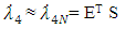
Within the performance index presented in (1), the functions and denote the control strategies employed by players and respectively; the function represents the immediate reward for player and signifies the terminal reward. Each player’s objective is to optimize their respective performance indices through the strategic selection of their control actions where ranges from 1 to 4.

The concept of an open-loop strategy refers to the predefined trajectory of a player’s actions over time [23]. This equilibrium notion is known for its temporal consistency, implying that no player has a reason to stray from their initial strategy as the game progresses. Consequently, we define an open-loop solution concept (equilibrium) as:

2.2. Definition

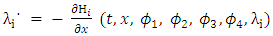
The collection of functions for each in 1, 2, 3, 4, constitutes an (OLNE) if, for any given , there is an optimal control trajectory that resolves problem (1) and corresponds to the open-loop Nash strategy [1].

The (OLNE) is defined by establishing Hamiltonian expressions to formulate the necessary first-order conditions for optimality in nonzero-sum differential games, indicated as (1). These expressions are introduced as follows [24]:

(2)

for each within the set {1, 2, 3, 4}. Here, the variables where spans from 1 to 4, are known as the adjoint or costate variables that are paired with the state variable .

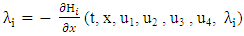
For the sake of brevity in the Hamiltonian formulations, the time dependency in the variables has been omitted.

Given that all functions in (1) possess continuous derivatives, the primary conditions for an optimal solution are provided by the Pontryagin’s Maximum Principle.

The Pontryagin’s Maximum Principle outlines the necessary conditions for an (OLNE) in a nonzero-sum differential game as follows:

(3)

(4)

(5)

accompanied by the initial and terminal conditions:

for every in {1, 2, 3, 4}.

From the stationary condition (5), the control is derived as where ranges from 1 to 4. Substituting this control into equations (3) and (4) leads to a set of differential equations solely in terms of and

(6)

(7)

with their respective boundary conditions:

(8)

(9)

and with denoted as for each within 1, 2, 3, 4.

In general, this set of Four-Point Boundary Value Problems (FPBVPs) tends to be nonlinear with mixed boundary conditions, making the precise analytical solution for the (OLNE) a complex task. This complexity necessitates the use of a suitable numerical technique for resolution.

3. Application of the Tau Technique in Multi-Player Differential Games

This section details how the Tau technique can be utilized to solve the system of FPBVPs to ascertain the (OLNE) in a four-player nonzero-sum differential game.

This method pivots on representing the function in as a truncated series in the form:

where denote the Jacobi polynomials, while are the corresponding spectral coefficients.

It should be noted that the omission of the temporal variable in subsequent discussions is meant for simplification. [25]

3.1. Definition

The set of Jacobi polynomials for , is defined as a series of orthogonal polynomials over the interval [−1, 1] against the weigh.

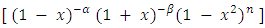
with . The explicit form of these polynomials is given by the Rodrigues formula:

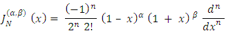
These polynomials encompass the Legendre polynomials for , the Chebyshev polynomials of the first and second kind for and , respectively.

3.2. Theorem

Given within (a Sobolev space), the closest approximation.

in the norm satisfies

where is a constant that depends only on the chosen norm, not on or .

Proof. Start by defining the Jacobi polynomial as follows:

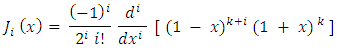Next, we’ll use the properties of Jacobi polynomials to expand the error term as a series of Jacobi polynomials:

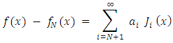Where are the expansion coefficients given by:

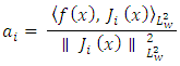Here, 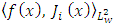w represents the inner product of and in the norm, and is the norm of in the norm.

Now, we’ll use the Sobolev space property to estimate 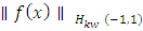. The Sobolev norm is defined as:

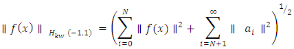Using Cauchy-Schwarz inequality, we can bound as follows:

Combining the expressions from the previous steps, we get:

We can bound using properties of Jacobi polynomials and . Since are orthogonal with respect to the weight function in the norm, we have:

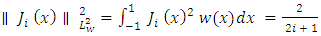Plugging this result into the previous expression, we get:

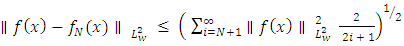Now, we can estimate the sum in the above expression by an integral:

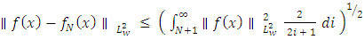Since , we have which means that is bounded by .

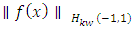Finally, we can simplify and bound the expression:

This establishes the desired inequality:

Where and the constant depends only on the chosen norm, not on or . This completes the proof of Theorem 3.2.

As per Theorem 3.2, the convergence rate of the Jacobi polynomial approximation is . The core principles and the convergence properties of the proposed method derive from the Jacobi Polynomial Approximation Theorem.

3.3. Theorem

(Jacobi Polynomial Approximation Theorem) For any function f in .

and as a natural number, there exists a unique polynomial approximation , the polynomial space of degree at most N with Jacobi polynomials, that minimizes the norm:

where is defined in terms of the orthogonal Jacobi polynomials as:

Here, the coefficients are determined by the inner product of and the Jacobi polynomials:

Proof. We aim to prove the existence and uniqueness of a polynomial in that minimizes the norm using Jacobi polynomials. We express as a linear combination of the Jacobi polynomials up to degree , i.e., 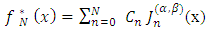. To minimize , where

we leverage the orthogonality property of Jacobi polynomials: if then and if then By taking derivatives with respect to and setting them equal to zero, we find , yielding coefficients that minimize the norm and provide . To establish uniqueness, assuming two polynomials and minimizing , we observe . After repeating the minimization process, we find that the coefficients for both polynomials are identical, confirming the uniqueness of the approximation.

To adapt the Jacobi polynomials for the interval the domain is transformed by:

We approximate the solution functions and , with , for the FPBVPs by a sum of shifted Jacobi polynomials:

(10)

(11)

(12)

(13)

(14)

where and are coefficients to be determined, and 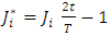for denote the shifted Jacobi polynomials on the interval [0, T].

The approximate values for the first derivatives of and with ranging from 1 to 4, are represented as:

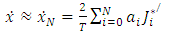(15)

(16)

(17)

(18)

(19)

These approximations can be reformulated in a vectorized manner as:

(20)

(21)

(22)

(23)

(24)

(25)

(26)

(27)

(28)

(29)

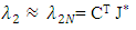
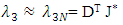
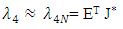
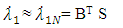
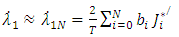
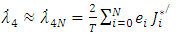
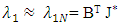
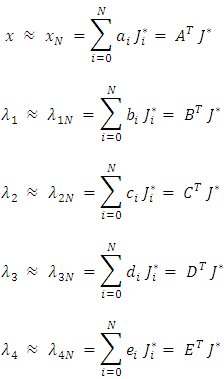
where and denote the coefficient vectors, J^* is the vector of modified Jacobi polynomials, and S represents the scaled derivatives of these polynomials.

In the Tau method, one integrates these equations, substituting Equations (20) through (29) into the original differential equations to construct the residuals:

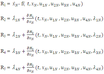These residuals are minimized by multiplying them by and integrating over the interval setting the result to zero, which leads to an algebraic system:

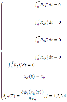The coefficients of the vectors and are determined by solving this system.

4. Exemplary Demonstration

This part evaluates the application of the Jacobi polynomial approach (JTM) on a bioeconomic model’s differential game to assess the method’s precision and computational effectiveness. In this ecological-economic context, four companies competitively exploit a shared regenerative natural asset (consider a fisheries scenario, for instance).

The rationale for choosing this particular bioeconomic framework is its complex nonlinear structure of (FPBVPs). This complexity is more pronounced than in several other economic models, such as those involving strategic marketing decisions like in Sorger [26]. Such complexity provides a robust test for the JPA’s precision and computational efficiency.

We define the temporal evolution of the shared renewable resource’s population within the time span via the subsequent state dynamic and initial state expression [27]:

where the smooth function 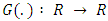signifies the resource’s intrinsic proliferation rate, taking the logistic growth form as

with r embodying the intrinsic proliferation rate and k the environment’s carrying threshold. Here, is the population magnitude of the resource at any time , while and represent the respective harvesting efforts of the enterprises at any given time , and and are the catch efficiency parameters.

For any enterprise from the set {1, 2, 3, 4}, the cumulative benefit throughout the interval is stated a

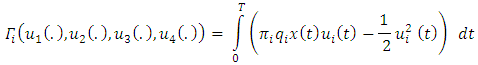where denotes the per-unit revenue from the resource for the firm. The term is indicative of the cost incurred due to harvesting at the effort [27].

To deduce the Nash equilibria for the companies in this ecological-economic interaction, the Hamiltonian for each firm is formulated as:

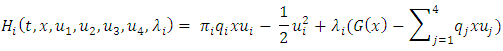Minimizing 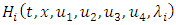with respect to gives the (OLNE) for each entity as:

(30)

The adjoint dynamics for the agent is given by:

(31)

where, upon substituting equilibrium strategies, one obtains a system of differential equations governing each .

The FPBVPs for this differential game are characterized by a series of equations corresponding to state, control, and adjoint variables for every firm .

Assume that the state equation’s unique trajectory, respecting the initial condition, is signified by , and the unique solutions of the adjoint dynamics conforming to the terminal conditions are , and , each pertaining to an individual competitor.

According to the ensuing theorem, these conditions uniquely describe the (OLNE) for the quartet of players in the presented bioeconomic game.

4.1. Theorem

The exclusive (OLNE) for the described differential game is uniquely determined by

(32)

(33)

(34)

(35)

Proof. For preset control actions , where we consider the following optimal control formulations:

• For competitor 1:

under the constraint:

• For competitor 2:

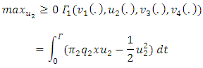with the boundary condition:

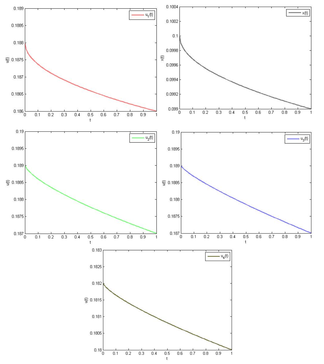Figure 1. Plots of approximate (OLNE) for exemplary demonstration when N = 14

The behavior and constraints for competitors 3 and 4 follow suit.

For each participant the integrand of the performance measure demonstrates concavity as a function of indicated by: .

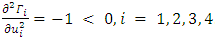The remaining part of the proof would similarly address the calculations for the other competitors [28].

The system of FPBVPs constitutes a series of nonlinear differential equations with segmented boundary conditions which usually do not permit an analytical solution. The parameters for a standard scenario are provided as:

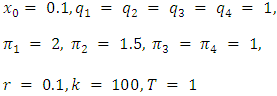This system of FPBVPs also incorporates the equations for and

To resolve these FPBVPs, we consider approximations for 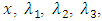and

In this approximation, represents the column vector of shifted Jacobi Polynomials.

For , representing the differential equation of

For expressing the dynamics of

For depicting the evolution of

For which constitutes the differential equation for

wherein and are specific constants akin to those in preceding formulae. For the differential equation for

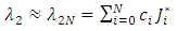
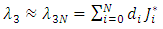
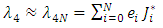
where and are constants, consistent with the framework of earlier equations.

The numerical outcomes for the optimal payoff functions , and with varying values are presented in the following tables. The graphs of approximate solutions for (OLNE) for are given in Figure (1).

Table 1. Optimal payoff function       for the four-player illustration with JTM

5. Conclusions

This research marks a significant stride in the field of economic game theory and computational economics by introducing an efficient algorithmic approach through the (JTM) method. By demonstrating the JTM’s capability to solve complex differential games more accurately than traditional methods, this paper contributes to the precision of economic forecasts and decision-making processes. The implications of these findings have the potential to refine economic models, optimize market strategies, and improve regulatory policies. Looking ahead, the application of JTM could catalyze advancements in financial engineering, market analysis, and resource management, shaping the future of economic theory and practice.