Shahd H. Alkharaz1, Esam A. El – Siedy1, Eliwa M. Roushdy2, Muner M. Abou Hasan3
1Department of Mathematics, Faculty of Science Ain Shams University, Egypt
2Department of Basic and Applied Sciences, Arab Academy for Science, Technology and Maritime Transport, Cairo, Egypt
3School of Mathematics and Data Science, Emirates Aviation University, Dubai, UAE
Correspondence to: Shahd H. Alkharaz, Department of Mathematics, Faculty of Science Ain Shams University, Egypt.
| Email: |  |
Copyright © 2024 The Author(s). Published by Scientific & Academic Publishing.
This work is licensed under the Creative Commons Attribution International License (CC BY).
http://creativecommons.org/licenses/by/4.0/

Abstract
This study delves into the application of differential games in marketing, emphasizing their role in formulating advertising and pricing strategies. By examining the Nash equilibrium, the research highlights the complexities and strategic implications of dynamic pricing in competitive markets. The study also presents a practical example and numerical analysis to demonstrate the real-world applicability of these theoretical models.
Keywords:
Differential Games, Marketing Strategies, Nash Equilibrium, Pricing Strategy, Advertising, Dynamic Market Analysis
Cite this paper: Shahd H. Alkharaz, Esam A. El – Siedy, Eliwa M. Roushdy, Muner M. Abou Hasan, Strategic Market Dynamics: Exploring Differential Games in Marketing and Pricing Strategies, Journal of Game Theory, Vol. 13 No. 1, 2024, pp. 1-6. doi: 10.5923/j.jgt.20241301.01.
1. Introduction
Differential game theory, an extension of traditional game theory into dynamic and continuous-time scenarios, is crucial in analyzing dynamic markets. This advanced mathematical framework employs differential equations to model continuous strategies and interactions among players, such as firms and consumers, over time. Its applications in dynamic markets include modeling market competition, understanding demand and supply dynamics, and analyzing innovation and technology adoption. In marketing science, it's instrumental for strategic decision-making, predicting market trends, and optimizing the marketing mix, especially in uncertain environments. It allows firms to develop adaptive strategies that adjust to fluctuating market conditions. While offering insights into scenarios like pricing wars and advertising battles, its practical application is often challenged by mathematical complexity and extensive data requirements, underscoring its importance yet highlighting its limitations in dynamic market analysis and marketing decision-making. The paper begins by introducing differential games as a crucial tool in marketing, especially in the context of dynamic market conditions and oligopolistic competition. It sets the stage for a detailed examination of how these games can model and predict market behaviors in advertising and pricing strategies ([1]-[3]).In the last three decades, differential games have emerged as a significant tool in the field of marketing science. This approach, blending dynamic optimization with game theory principles, is particularly relevant due to two main characteristics of markets: their dynamic nature and the prevalence of oligopolistic competition. Differential games enable marketers to analyze and anticipate outcomes in a setting characterized by both competitive and evolving aspects.This tutorial is designed to acquaint readers with the fundamental principles of differential games and to explore various models that have been applied in the marketing domain. Additionally, it demonstrates the real-world relevance of these models. The focus here is not to exhaustively cover all aspects of differential games in marketing, as comprehensive treatments are available in works by Jørgensen and Zaccour [4], Erickson ([5]-[8]), and Dockner et al [9]. The paper further explores Nash equilibrium in the context of pricing strategies, detailing methods to develop such strategies and their numerical analysis using MATLAB. It also addresses the concepts of time consistency and subgame perfectness in pricing strategies, illustrated with practical examples, before concluding and referencing relevant literature.
2. Core Principles of Differential Game Theory
Differential games operate in a framework of continuous time, involving two primary categories of variables: the decision variables and the state variables. In a marketing context, the decision variables can include factors like advertising investment and product pricing, while state variables represent the resulting market metrics such as sales volume or market penetration. These variables are all time-dependent, necessitating that each participant in the game strategizes a trajectory of decision variable values over a given period, with state variables evolving in tandem due to the influence of these decisions.Let  symbolize time, and assume the presence of
  competitors in the game, with
  being an integer no less than 2. For each competitor
  belonging to the set
  there exists a decision variable
  generally a vector, constrained by
  . The state of the game at any time
  is described by an m-element vector
  , with the initial state
  at
at  being predetermined and constant. The progression of the game state is governed by a set of differential equations:
  | (1) |
Here, the change rate of state variables is a function of time, the current game state, and the decisions made by the  competitors. The gain for each competitor
  at any given time
  is influenced by the time, the game state, and the decisions:
  | (2) |
Each competitor’s aim is to optimize the current value of their cumulative gains, formulated as: | (3) |
In this formula,  represents the discount rate of competitor i, and
  is the residual value for
  at the end of the period. The time frame
  can be unbounded
  , which eliminates the need for a residual value. With the inclusion of a pricing strategy, the decision variables are adjusted to integrate dynamic pricing mechanisms, which in turn affect the state variables, particularly in aspects like market share and revenue. Consequently, the equations and variables are tailored to accommodate these strategic pricing considerations within the differential game structure ([10]-[12]).
3. Nash Equilibrium with Pricing Strategy Integration
In this context, players decide on their strategies, including pricing, simultaneously, without forming binding agreements, and with complete knowledge of all objective functions. Each player understands that their competitors are also making control decisions, including pricing, to optimize their outcomes. A Nash equilibrium is reached when each player maximizes their payoff, considering the strategies, including pricing models, selected by other players. Formally, a collection of strategies  achieves a Nash equilibrium if the following condition is met for every player
  in the set
 | (4) |
Here,  represents the modified control action, which now includes a pricing strategy component. This change implies that the control variables
  are expanded to incorporate pricing decisions, influencing both the dynamics of the market (state variables
  and the players’ payoffs
  . The equations and symbols are thus adapted to encompass these strategic pricing considerations, ensuring alignment with the objectives and the competitive dynamics in the differential game scenario.The preceding paragraph discusses integrating pricing strategies into the concept of Nash Equilibrium within a differential game scenario. Here, "players" (or market competitors) simultaneously decide their strategies, including pricing, with full knowledge of everyone's goals and without forming binding agreements. A Nash equilibrium occurs when each player's strategy maximizes their payoff, considering others' strategies. Formally, this equilibrium is defined by a set of strategies where no player can improve their payoff by changing their strategy alone. The control actions now include pricing strategy components, expanding decision variables to cover pricing decisions, which affect market dynamics and individual payoffs. Consequently, the traditional mathematical equations and symbols in this context are adapted to include these strategic pricing considerations, ensuring they align with competitive market dynamics and objectives in such games.
4. Determination of Nash Equilibria with Pricing Strategy
To develop Nash equilibrium strategies incorporating pricing strategies, two approaches are typically employed: optimal control methods (involving Hamiltonians and costate variables) and dynamic programming principles (utilizing value functions and Hamilton-Jacobi-Bellman equations). Optimal control is suited for open-loop strategies including dynamic pricing, while dynamic programming is effective for feedback strategies that adjust prices based on market state [13].The optimal control approach involves formulating a Hamiltonian for each player, incorporating the pricing strategy:  | (5) |
Here,  represents a vector of m costate variables, and the control variables ui(t) include pricing decisions. For time-only strategies, Nash equilibrium conditions (4) lead to these necessary conditions:
 | (6) |
These conditions, along with the state dynamics (1), form a two-point boundary value problem (TPBVP), solvable through numerical methods. For an infinite time horizon, the alternative transversality condition becomes: | (7) |
In feedback strategies involving pricing, the conditions for costate variables are: | (8) |
This situation is more complex due to the interdependence of strategies and state variables, making the system of equations (8), (1) challenging to solve. Employing the Hamilton-Jacobi-Bellman equation for dynamic programming, with value functions Vi(t, x) for players, leads to feedback equilibrium if: 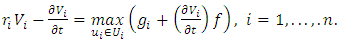 | (9) |
With boundary conditions for a finite horizon:  | (10) |
For an infinite horizon, the term  in equation (9) disappears, and the boundary condition is replaced by the boundedness of the objective functionals [9]. Although equations (9)–(10) are typically challenging to solve, certain models allow for discerning the functional form of value functions, facilitating a solution. The inclusion of pricing strategies in this framework requires modifying the control variables
  to encompass dynamic pricing, which affects the state dynamics, payoffs, and ultimately, the strategies for achieving Nash equilibrium
5. Time Consistency and Subgame Perfectness in Pricing Strategies
In dynamic noncooperative games with pricing strategies, two crucial requirements for Nash equilibria are time consistency and subgame perfectness. Consider a subgame  at some point
  defined over the interval
  with initial condition
  In this subgame, player i’s objective, inclusive of pricing strategy, is given by:
  | (11) |
with the system dynamics incorporating pricing decisions: | (12) |
The original game, as outlined in (1)–(3), is denoted by  . Time consistency implies that if
  is a Nash equilibrium of
  with a unique equilibrium state trajectory
  then for any
  the subgame
  must have a Nash equilibrium
  such that
  for all i in
  and
and  . This criterion ensures the Nash equilibrium is time consistent. Both open-loop and feedback Nash equilibria with pricing strategies satisfy this requirement. Subgame perfectness, a stronger condition, requires that for any
  the subgame
  has a Nash equilibrium
  with
with  for all
  and
and  . This ensures that the equilibrium is not only consistent over time but also perfect in every subgame. Feedback Nash equilibria with dynamic pricing are typically subgame perfect, but open-loop Nash equilibria may not be unless players can commit to fixed strategies, including pricing, at the game’s outset. The distinction lies in subgame perfectness requiring equilibrium within any
  , for all
  , beyond just the equilibrium state trajectory, as is needed for time consistency. The integration of pricing strategies adds complexity to these conditions, necessitating adjustments in both control actions and strategic considerations to maintain equilibrium in the dynamic market scenario.
6. Example with Pricing Strategy
An example, adapted from Kamien and Schwartz [14], demonstrates the determination of open-loop and feedback Nash equilibrium strategies incorporating pricing strategies. In this scenario, two competitors produce an identical product and need to develop strategies involving time-varying production schedules u1(t) and u2(t), as well as dynamic pricing. The production cost for each competitor is identical: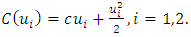 | (13) |
The competitors face a common price state variable p(t), evolving according to:  | (14) |
Here, s measures the price adjustment speed, accounting for demand and total quantity supplied. Each firm aims to maximize its discounted profit, incorporating pricing decisions:  | (15) |
Subject to the dynamic constraint (14).For the open-loop Nash equilibrium, form the Hamiltonians: 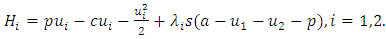 | (16) |
The necessary conditions are: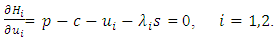 | (17) |
 | (18) |
 | (19) |
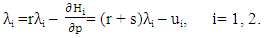
Solving (17) for  integrating (18) with an integrating factor, and applying (19), yields:
  | (20) |
From (17),  . Differentiating (17), substituting from (14), (18), and (17), yields:
  | (21) |
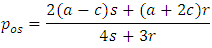
For steady-state open-loop strategies  , the output and price are:
 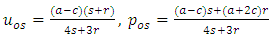 | (22) |
For feedback Nash equilibrium, consider the value function for each competitor: 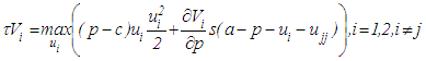 | (23) |
Maximizing with respect to  gives:
 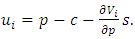 | (24) |
Substituting equation (24) into (23) and incorporating a pricing strategy, we get: 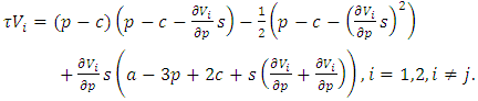 | (25) |
Here, the partial derivatives for both competitors appear. We seek interior solutions, ensuring  , under the assumption that
  . The system of equations (25) is solved to find the value functions V1 and V2. We conjecture the following quadratic functions:
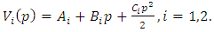 | (26) |
This implies: 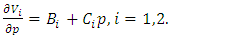 | (27) |
To ensure that the value functions (26) are solutions to (25), the constants  and coefficients
  and
and  must satisfy certain values. By substituting (26) and (27) into (25), we get:
 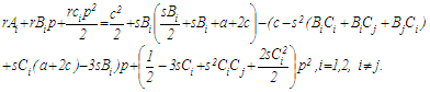 | (28) |
Equating coefficients of  in (28):
 | (29) |
Equating coefficients of  gives expressions for
  in terms of
  and equating constant terms provides expressions for
  as functions of
  To establish that
  we subtract the two equations in (29):
  | (30) |
It follows that either  or:
or: 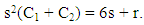 | (31) |
Substituting from (27) into (24) and then into the state equation (14):  | (32) |
The solution to (32) is: | (33) |
For p(t)to converge as t → , s(C1+C2) < 3 or s2(C1+C2) < 3 is required. However, from (31), this implies 3s + r < 0 which is not possible as both
  and
and  are nonnegative. This rules out an asymmetric equilibrium. Establishing C1 = C2 = C we solve for roots from (29):
 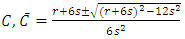 | (34) |
To choose between the roots, we consider (33). For convergence, 2sC -3 < 0 or  is required. The larger root,
  exceeds this limit, preventing convergence. Only the smaller root allows for the convergence of
  From (28):
 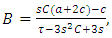 | (35) |
where  is the smaller root. The feedback Nash equilibrium production strategy is:
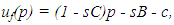 | (36) |
yielding the steady-state price: 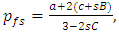 | (37) |
and steady-state output for each competitor: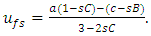 | (38) |
Feedback strategies differ from open-loop strategies, leading to distinct long-term outcomes.
7. Numerical Analysis
Using MATLAB, we perform a numerical analysis for both open-loop and feedback Nash equilibrium strategies with the following parameter values:• Demand parameter,  • Cost parameter,
  • Speed of price adjustment,
  • Discount rate,
  • Initial price,
7.1. Open-loop Nash Equilibrium
The open-loop Nash equilibrium is determined using equations: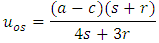
7.2. Feedback Nash Equilibrium
For the feedback Nash equilibrium, we first solve the quadratic equation (29) to find the smaller root C. We then use C to calculate B using equation (35), and finally compute ufs and pfs using equations (36) and (37).
7.3. Results
The calculated values are: • Open-loop Nash equilibrium: - Steady-state output, uos: 2.087 units - Steady-state price, pos: 5.826 units • Feedback Nash equilibrium: - Steady-state output, ufs: 2.053 units - Steady-state price, pfs: 5.335 units - Smaller root  from Equation (29): 0.331 These results demonstrate that the steady-state outputs and prices in the feedback Nash equilibrium strategy differ slightly from those in the open-loop Nash equilibrium strategy, a common characteristic in dynamic game scenarios as in Figure 1.
 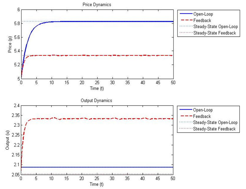 | Figure 1. Comparative Analysis of Open-Loop and Feedback Nash Equilibrium Strategies |
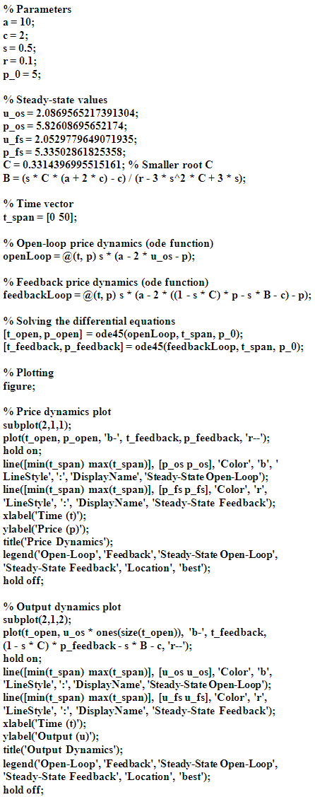
8. MATLAB Code Used in the Example
9. Conclusions
The study concludes that differential games offer significant insights into marketing strategies, particularly in dynamic pricing and advertising. The numerical analysis and practical example provided reinforce the applicability of these theoretical models in real-world scenarios, offering valuable tools for marketers to navigate competitive landscapes.
References
| [1] | G. E. Fruchter. The many-player advertising game. Management Science 45:1609–1611, 1999. |
| [2] | G. Sorger. Competitive dynamic advertising: A modification of the Case game. Journal of Economic Dynamics and Control 13:55–80, 1989. |
| [3] | M. L. Vidale and H. B. Wolfe. An operations-research study of sales response to advertising. Operations Research 5:370–381, 1957. |
| [4] | S. Jørgensen and G. Zaccour. Differential Games in Marketing. Kluwer Academic Publishers, Boston, MA, 2004. |
| [5] | G. M. Erickson. Dynamic Models of Advertising Competition, 2nd ed. Kluwer Academic Publishers, Boston, MA, 2003. |
| [6] | G. M. Erickson. Empirical analysis of closed-loop duopoly advertising strategies. Management Science 38:1732–1749, 1992. |
| [7] | G. M. Erickson. Dynamic Models of Advertising Competition, 2nd ed. Kluwer Academic Publishers, Boston, MA, 2003. |
| [8] | G. M. Erickson. Advertising competition in dynamic oligopolies. Working paper, University of Washington Business School, Seattle, WA, 2007. |
| [9] | E. Dockner, S. Jørgensen, N. Van Long, and G. Sorger. Differential Games in Economics and Management Science. Cambridge University Press, Cambridge, UK, 2000. |
| [10] | J. H. Case. Economics and the Competitive Process. New York University Press, New York, 1979. |
| [11] | R. Davidson and J. G. MacKinnon. Several tests for model specification in the presence of alternative hypotheses. Econometrica 49:781–793, 1981. |
| [12] | K. R. Deal. Optimizing advertising expenditures in a dynamic duopoly. Operations Research 27:682–692, 1979. |
| [13] | G. E. Fruchter and S. Kalish. Closed-loop advertising strategies in a duopoly. Management Science 43:54–63, 1997. |
| [14] | M. I. Kamien and N. L. Schwartz. Dynamic Optimization: The Calculus of Variations and Optimal Control in Economics and Management, 2nd ed. North-Holland, Amsterdam, The Netherlands, 1991. |

 Abstract
 Reference
 Full-Text PDF
 Full-text HTML