1. Introduction

In game theory, Nash equilibrium is one of the most well-studied solutions to a single-stage non-cooperative game. An equilibrium in the game is defined as no player can do better by unilaterally changing his strategy. It is proved that if mixed strategies are allowed, then a game with a finite number of players and finitely many pure strategies has at least one Nash equilibrium [1]. The problem of finding equilibrium in various single-stage game settings has been studied in the literature.

In reality, dynamic game playing over time is more complex than one game. Instead, decision-makers are expected to play one game followed by another, or maybe several other games. It is tempting to view each game independently and assume players do not make any attempt to link them. If each player treats every game independently, equilibrium can be studied for each of the stage games in turn. However, this approach ignores any real issues concerning sequential behavior, if we consider the games played sequentially as stages of a larger game and players can observe the outcomes of each game before another game is played. If players are rational and forward-looking, they should view the sequence of decision-making as part of one large game. And if they do, we expect their actions to be dependent on the outcome of the previous games.

The existence and solutions of equilibrium for dynamic games are well-studied in the literature. The existence of sub-game equilibria in simultaneous move games with finite actions was discussed by Fudenberg and Levine 1983 [2]. Kreps and Wilson [3] proposed the concept of sequential equilibrium and Myerson [4], in his key paper in 1986, discussed the sequential communication equilibrium in multi-stage games with communication mechanisms that can be implemented by a central mediator. There has been a surge of discussions in multistage game playing with various designs of dynamic mechanisms and information systems. For example, Renault, Solan, and Vieille [5] studied a dynamic model of information provision with a greedy disclosure policy, and He and Sun [6] discussed the existence of subgame-perfect equilibria in dynamic games with simultaneous moves.

In this paper, we discuss details of conditional decision-making in a multi-stage game with players choosing their actions simultaneously at each stage. Games at each stage are played sequentially, with actions and information from previous games unfolding, but the payoffs were delayed until the sequence ends. These games form a general class of dynamic games with many applications in economics and political science. We define the settings of a multi-stage game and its equilibrium in section 2. The existence of equilibrium in this game setting is discussed through the idea of backward induction in section 3. An example of a simple game with two players and two stages is presented in section 4. Concluding remarks are discussed in section 5.

2. The Setting of a Multi-Stage Game

Consider a multi-stage game with players and finite stages. At each stage, player , has a finite strategy space . Let denote the pure strategy chosen by player at stage . Then is the profile of strategies used by each player at stage , where . Assume the game at each stage is a simultaneous move game, i.e a normal-form game.

At stage , the outcome for player is denoted by and the combined outcome for all players is denoted by vector . Assume the combined outcome at stage comes from a joint distribution that is known given the joint choice of actions, i.e. , where depends on the joint action .

Assume each game is played in a distinct period and also that after each stage is completed, all players observe the outcome of that stage and all outcomes gained before that stage, i.e. are observed for each player at stage . It is plausible that the action of each player at stage will depend on the observed outcome at previous stages. In this setting, the outcomes of previous stages become common knowledge, and players are allowed to make conditional strategies for future games based on past outcomes.

2.1. The Payoff

The games are played sequentially, and the total payoffs from the sequence of games will be evaluated using the sequence of outcomes at the end of the games, i.e. after stage . Suppose each player receives a real number payoff or reward. The reward function for player is defined as a function of the outcomes of all stages, i.e. . The joint reward function for all players is then defined as , where . With the reward function defined, the expected reward of each player can be calculated when the joint strategies at all stages are given.

Given the joint actions at all stages , the expected reward for player is defined as

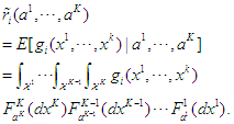
2.2. Mixed Strategy

In a general setting, at a given stage, each player is allowed to have mixed strategy, i.e. players choose actions based on a probability distribution of possible pure strategies at the stage. Consider the decision function for player at stage , , as a function from the product space of the previous outcome space 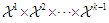to the probability space of strategies at stage . And the joint decision function for all players at stage is then denoted by 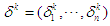, where .

Assume the joint reward 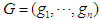at the end of the game is defined the same as above. Given the joint mixed strategies at all stages, 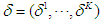, the expected reward for player is can be calculated as

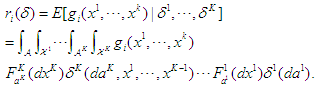
2.3. Definition of Equilibrium

In a single-stage game, the Nash equilibrium is achieved when no player can increase his own expected payoff by switching his strategy. A collection of mixed strategies for all players, , is considered to be the equilibrium strategies if for all ,

where denotes a new set of mixed strategies when only player switched from mixed strategy to .

Due to the multi-stage nature of the game, the decisions for all players are made stage by stage based on the previously observed outcomes. The equilibrium joint strategies of the game is thus defined sequentially as no players can be better off by switching to another strategy at each stage conditionally on observed previous outcomes. The joint mixed strategies for all players at all stages 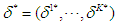, is considered to be an equilibrium if at any stage given outcomes from stage 1 to , for all player . The expected reward of player at the equilibrium satisfies the following,

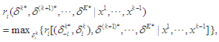where denotes a new joint randomized decision at stage k when only player switched from to .

3. The Existence of Equilibrium

It has been shown that there is a Nash equilibrium for every single-stage finite game when mixed strategies are allowed. The proof of existence is outlined in Nash's original paper using Kakutani fixed-point theorem [7]. We now extend the discussion to a multi-stage game using the idea of dynamic programming and backward induction, which was developed by Richard E. Bellman [8]. The essence of dynamic programming is to simplify a complicated optimization problem by breaking it down into simpler sub-problems recursively. The nature of a multi-stage game allows us to break the game down into a sequence of sub-games over discrete time, with each sub-game as a finite non-cooperative game. Starting from the end of the game, we first examine the last stage and identify what strategy would be most optimal at that moment. We then backtrack and determine what to do at the second-to-last time the decision. This process continues backward until one has determined a sequence of optimal actions for every possibility at every point.

Consider the last stage, stage , of the game when the outcomes of the previous stages are observed. The expected reward based on the joint decision of all players at the last stage, , is given by

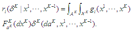When the outcomes from stage 1 through , i.e. are observed, the game at the last stage becomes a single stage game, which has an equilibrium as proved by Nash [7]. Denote the equilibrium decision at stage based on previous observations as and the equilibrium expected reward given outcomes from stage 1 to is given by 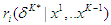. If the players follow the equilibrium strategy 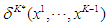at stage K, then the expected reward can be written as

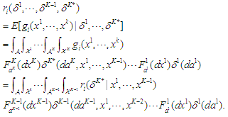Assume all players follow joint strategy at stage , now consider stage given the information of previous outcomes up to stage . The expected reward is then given as

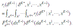This again becomes a single-stage game, and Nash equilibrium exists. Denote the equilibrium decision at stage as 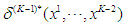and the equilibrium expected reward given outcomes from stage 1 to is given by 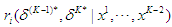. Repeat the process sequentially for stage . We can then find an equilibrium decision for all stages, .

4. An Example

4.1. A Game with 2-Stages

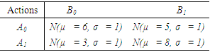
Consider a simple game with players and stages. Players are non-cooperative and play simultaneously. Player has 2 pure strategies to choose from at each stage, denoted by and . Similarly, player also has 2 possible pure strategies, and . Assume the outcomes for player A and B are the same at each stage, and follow a distribution , if player choose pure strategy and player choose pure strategy at the stage, i.e. Assume mixed strategies are allowed. Let denote the probability of player A choosing pure strategy and be the probability of player B choosing strategy .

4.2. The Reward Function

Consider the zero-sum game, in which the sum of rewards for players and player equals zero. Consider the situation that the goal of player in this game is to reach a threshold and the opponent wants the opposite. Furthermore, assume the game stops whenever the threshold is achieved. Thus, the reward function at the end of the game is given by

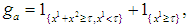where . The expected reward function is then given by

where .

4.3. Computing the Mixed Equilibria

We compute the mixed equilibrium strategy through backtracking. Start with stage 2 given the outcome in stage 1 and assume the threshold has not been achieved, i.e. is known and less than . The expected reward for player A is then given by

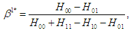
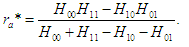
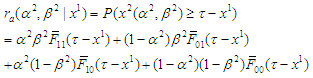Now the problem at stage 2 becomes a single-stage zero-sum game, where the equilibrium can be obtained using the min-max decision rule (see, for example, [9]). The optimal strategies and the corresponding equilibrium at stage 2 are given by

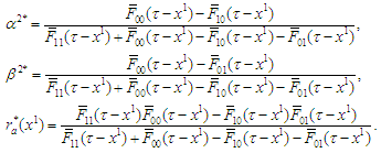Now consider the first stage assuming the players follow the optimal strategies given above at the second stage.

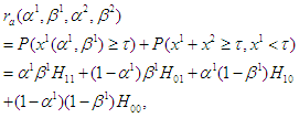where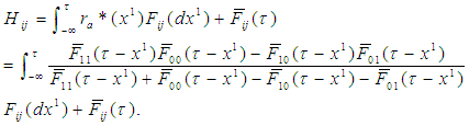

Now the game again becomes a single-stage zero-sum game, where the equilibrium can be obtained as follows

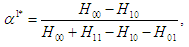(1)

(2)

(3)

4.4. Numerical Calculation and Simulation

Assume the outcomes for players A and B are the same at each stage and follow normal distributions (with different means and standard deviation 1). The distributions of the outcomes for each combination of actions are listed in table 1. Assume mixed strategies are allowed. The goal of player in this game is to reach a threshold and the opponent wants the opposite. The game stops whenever the threshold is achieved. The expected reward for player A is then given by .

Table 1. The distributions for the random outcomes in each joint action

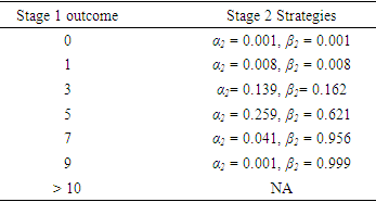
Following the calculation in the previous section, the expected reward for player A under equilibrium is 0.688 (equation (3)), and the equilibrium mixed strategies in stage 1 are given by and (equation (1) and (2)). The integrations in the calculation of are numerical approximations since the integrals can not be obtained in closed form. The strategies of both players A and B in stage 2 will vary depending on the outcome from stage 1. Table 2 listed some examples of strategies played in the second stage. In the last example, since the goal has been achieved in stage 1, the game stopped without going into the second stage.

Table 2. Mixed strategies played in stage 2 under different stage 1 outcomes

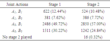
A simulation study was performed, with 5000 such games played. In this simulation, player A reached the goal () for 3438 games which are 68.94% out of 5000 games. The number of times and the proportion of each joint action played at each stage are listed in Table 3.

Table 3. The number of times each joint action played at each stage in 5000 simulated games

5. Discussion and Remarks

In this paper, we focus on conditional decision-making in a multi-stage game with players choosing their actions simultaneously in the absence of coalitions. We defined and showed the existence of the multi-stage equilibrium. We also provide algorithm steps toward the calculation of such equilibrium using dynamic programming. Opposed to the traditional non-cooperative game setting, the joint actions of a cooperative multi-stage game can also be studied. In fact, John von Neumann and Morgenstern [10] presented a theory that analyzes various of types of coalitions that can be formed. A prefigured discussion of backward induction in a 2-person zero-sum setting is provided in their book.

The multi-stage game setting discussed in this paper assumes a simultaneous game at each stage, i.e. player chooses their action without knowledge of the actions chosen by other players. Sequential behavior within a stage can also be added to the game setting, which allows the possibility that players to move in turns in each sub-game. The sequential game at each stage can be analyzed mathematically using combinatorial game theory. Equilibrium can be found using backward induction if perfect information is assumed [11]. Sequential playing simply adds an additional layer to the current dynamics.

Perfect information about outcomes at previous stages is assumed in the setting of a multi-stage game. However, it is possible to imagine a game where some stages are played before the outcomes of previous stages are observed. If no information from previous stages is observed at all, the game at each stage can be treated as no different from a single-stage simultaneous game. If some, but not all the information is revealed, the analysis can become complicated depending on the structure of the information. If not all players are conscious of the other players' actions and payoffs at each stage, the backward induction analysis will not be easily applied [12].