1. Introduction

One starts from the notion of “monopolistic competition”. It was very popular among economists in the 30’s. It is a trade-off between the interests of the firms and consumers. Thanks to differentiated products the firms can choose high enough prices and their profits are sufficient. Concerning the consumers, they benefit from diverse products. More accurately, “monopolistic competition” is between “perfect differentiation of the products” and “price war”.

- “Perfect differentiation of the products” means separate markets. Each firm chooses the monopoly price. There is no effect on the customers of a firm, of the prices chosen by the other firms. It is favorable to firms, which can choose enough high prices.

- “Price war” means that the products are not enough differentiated, and this makes each firm decrease its price to get customers. Finally, the prices are low and the firms make no profit. It has been described as the Bertrand paradox [1]. Of course, it is favorable to consumers.

“Monopolistic competition” means that the products are partially substitutable and enough differentiated. The important idea is: each firm has its “garden” (or captive customers), customers that the firm is sure to keep (even if there is a condition on the price, which should not be too high). At the equilibrium, each firm has chosen a not too high price, and benefits from its “garden”. Therefore, the profits are sufficient.

Unfortunately, the two models of “monopolistic competition”, the Chamberlain’s one and the Hotelling’s one, were … erroneous [2]. It has been demonstrated later. When one applies the definition of Nash equilibrium very accurately, one demonstrates that the models were erroneous. Tirole, a French economist who was awarded the Nobel prize of economics, demonstrated that there was an error in the Chamberlain’ model [2]. And researchers demonstrated that the Hotelling’s model was erroneous [3].

In this article one proposes a new definition of “monopolistic competition”. The method is Bertrand competition, the demands being deduced from the consumers ‘utilities [4]. The “garden” of a firm E_i is the consumers with a utility u_i = 1, if 1 is the maximal price. Each firm keeps the consumers in its garden, provided that its price is the lowest (for instance, if the prices are equal, each firm has for customers exactly the consumers in its garden). To simplify, one considers only three competitors and one supposes that the costs are equal to 0.

The plan of the paper is:

- First, one sets out the method which is used.

- Then one studies the mathematical properties of the “monopolistic competition”. One demonstrates the existence of a Nash equilibrium, thanks to the Sperner’s lemma. One shows that the characteristics of product differentiation are described by the model.

- One has to define “disruption”. The disruption is when one of the firms increases the utility of the consumers in its “garden”. For instance, E₁ is disruptive if the utility for the consumers in its garden increases from 1 to 1, 5, while u₂ = 1 and u₃ = 1. In the general case, when a firm E_i increases the utilities of the consumers u_i from u_i to u_i + k (k > 0) its profit P_i increases. One demonstrates it. However, in the particular case of “monopolistic competition” there is a difficulty. One has to set out another demonstration.

- One presents two tractable examples.

- A goal of the paper being to explore the possibilities of the model used, one quotes some results already achieved. They concern the profitability of mergers of some kind, when the bought asset is closed down after the merger. The model can be used also to show that there are two kinds of innovation: non differentiating innovation and differentiating innovation. And it can be used to study the role of cannibalization.

- A tractable example is presented, showing the role of cannibalization. The question which is posed is the best choice for a firm which wants to disrupt: before disruption, it can buy and manage a competitor, or buy and close down it, or make no purchase.

- In the Conclusion one tries to explain why disruption is an attractive choice for entrepreneurs. Also, one considers the possible following of these works.

2. The Method

One uses the model of Bertrand competition the demands being deduced from the utilities of the consumers. This method has already been used by the author in several articles [4].

The utilities for the consumers of the three products sold (u₁, u₂, u₃) are in a cube 0 ≤ u_i ≤ 1. For prices (p₁, p₂, p₃) (0 ≤ p_i ≤1) the demand D_i corresponds to a “pocket” where are the consumers preferring the product of E_i and buying it. For instance, for E₁ the conditions are:

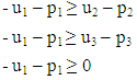(1)

After, the formulas for the profits are obvious:

P_i (p₁, p₂, p₃) = p_i D_i (p₁, p₂, p₃)

There are several interesting mathematical relationships:

(2)

(3)

It means that to calculate the variation of the consumers ‘surplus between two points M (p₁₀, p₂₀, p₃₀) and M’ (p’₁₀, p’₂₀, p’₃₀) one can integrate dS = -∑ dp_i D_i alongside any path from M to M’.

(4)

It is easily demonstrated using (1) and supposing an increase dp₁ = dp₂ = dp₃ = dp ≥ 0. The demand D₁ decreases.

(5)

To prove the existence of a Nash equilibrium one can use the Poincaré Miranda theorem.

The function (∂P₁ / ∂p₁, ∂P₂ / ∂p₂, ∂P₃ / ∂p₃) has positive values for the coordinate ∂P_i / ∂p_i in the internal facet u_i = 0 and negative values in the external facet u_i = 1. That ∂Pi / ∂pi has a negative value if u_i = 1 is a consequence of the conditions C₁ and C₂. It is explained later in the paper. Therefore, there is at least one point where the function is equal to 0: ∂P_i / ∂p_i = 0. It is a Nash equilibrium if the second order condition is fulfilled.

One has to make hypotheses. For instance:

C₁: for any price p_i fixed, the two other prices varying, the prices are strategic complements.

C₂: there is a unique (stable) equilibrium

C₃: the second derivatives ∂²P_i / ∂p_i∂p_j are negative (or equal to 0)

The condition C₃ implies C₂. So, one can choose (C₁, C₂) or (C₁, C₃). The point where ∂P_i / ∂p_i = O is a Nash equilibrium, since ∂²P_i / ∂p_i² ≤ 0 (condition C₁).

Notice that C₁ has for consequence that ∂P_i / ∂p_i is negative if u_i = 1. Indeed, it is the consequence of the existence of a reaction function: when the two other prices are fixed, when p_i varies from 0 to 1, ∂Pi / ∂p_i is positive at the start (p_i = 0) then decreases to 0 at the intersection with the reaction function and has a negative value when p_i = 1.

Also, the Jacobian which has for coefficients a_ij = ∂²P_i / ∂p_i∂p_j has a determinant which is negative. For instance, if the hypotheses are (C₁, C₂) one proves that the determinant is negative by adding the second and the third columns to the first one. One has: ∂²P₁ / ∂p₁² + ∂²P₁ / ∂p₁∂p₂ + ∂²P₁ / ∂p₁∂p₃ ≤ 0 using (2), (4) and (5) and supposing ∂²D_i / p_i² ≤ 0 (a sufficient condition to have ∂²P_i / ∂p_i² ≤ 0). The coefficients a_ii are negative and the a_ij are positive (because of C₁). The quantities a_ii a_jj – a_ij a_ji are positive (because of C₂). The determinant which is negative is a sufficient condition for the equilibrium being stable (for the small variations of the p_i). All these conditions are fulfilled when the demands are linear. The functions D_i can be any function differentiable twice. One has to suppose that the Nash equilibrium is unique.

3. Definition of the “Monopolistic Competition”

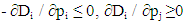
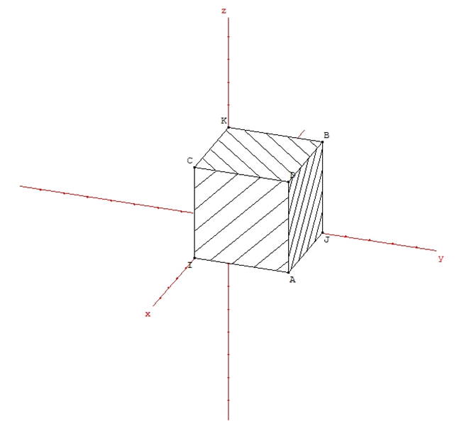
Each firm E_i has its garden, the consumers in the facet u_i = 1. All the consumers are in a garden.

One sets out the particular mathematical properties of the “monopolistic competition”. The property P₂ is very interesting from an economic point of view: it states that an equal increase of the prices does not change the demands. It shows why the “monopolistic competition” is advantageous for the firms: if they increase prices all together, no firm loses customers. For instance, in the symmetrical case, the prices can be 1, the maximal price, each firm keeps its “garden” (demand 1/3) and each profit is 1/3.

Also, one demonstrates that there is a Nash equilibrium, thanks to the Sperner’s lemma. It is not necessary, since the Poincaré Miranda theorem could be used (the “monopolistic competition” is a particular case of Bertrand competition). But it is interesting in itself, and allows to handle the mathematical properties of the “monopolistic competition”. These mathematical properties are useful to make some demonstrations, later in the paper.

These mathematical properties are:

P₁. For any (p₁, p₂, p₃), all the consumers buy some product. This is obvious. Any consumer belongs to the garden of a firm E_i. Therefore u_i - p_i = 1 - p_i ≥ O. This consumer buys the product of E_i, or another, if the net utility is more. Therefore D₁ + D₂ + D₃ is constant. If the sum which is constant is 1: D₁ + D₂ + D₃ = 1.

P₂. When (p₁, p₂, p₃) is changed in (p₁ + k, p₂ + k, p₃+ k) the demands remain the same. Take the example of D₁ and consider (1). The two first inequalities remain valid. Now, if a consumer buying the product of E₁ belongs to the garden of E₁, u₁ – p₁ = 1 – p₁ ≥ 0 remains valid. This consumer remains in the garden of E₁. If the consumer buying the product of E₁ belongs to the garden of E₂ u₂ = 1 and the first inequality u₁ – p₁ ≥ u₂ – p₂ = 1 – p₂ ≥ 0 shows that u₁ – p₁ ≥ 0. It is the same if the consumer belongs to the garden of E₃. Not only the demands but the first and second derivatives are constant when the prices increase of k. The demands are constant along a “ray” that is to say a segment parallel to the bisector (0, 0, 0), (1, 1, 1), linking an internal facet to an external facet. An example or ray is the segment (½, 0, ½), (1, ½, 1) (figure 1). One can choose a “basis” on a ray, some point M₀ and all the points on the ray are represented by a parameter x: OM= OM₀ + X, X being the vector (x, x, x). For instance, one can choose the middle of the ray described before, as a basis: M (¾, ¼, ¾). The parameter varies from -¼ to +¼. There is this mathematical relationship: ∂D₁ / ∂p₁ + ∂D₁ / ∂p₂ + ∂D₁ / ∂p₃ = 0 (and the same for j = 2 and j = 3).

P₃. The profit varies in a linear way along a ray. If a “basis” is chosen on the ray the price p_i varies from p_i0 + x₁ to p_i0 + x₂. Therefore, the profit P_i is P_i = (p_i0 + x) D_i. The demand D_i is constant. The profit varies in a linear way.

P₄ There is this mathematical relationship: ∂²D₁ / ∂p₁² + ∂²D₁ / ∂p₁∂p₂ + ∂²D₁ / ∂p₁∂p₃ = 0 (the same for j = 2 and j = 3) (6). Since D₁ is constant along a ray: ∂D₁ / ∂p₁ + ∂D₁ / ∂p₂ + ∂D₁ / ∂p₃ = 0. The relationship (6) is obtained by deriving in p₁. Also, ∂P₁ / ∂p₁ + ∂P₁ / ∂p₂ + ∂P₁ / ∂p₃ = D₁, deriving in p₁: ∂²P₁ / ∂p₁² + ∂²P₁ / ∂p₁∂p₂ + ∂²P₁ / ∂p₁∂p₃ = ∂D₁ / ∂p₁ < 0.

Now we can demonstrate the existence of Nash equilibrium using the Sperner’s lemma.

Figure 1. The cube 0 ≤ ui ≤ 1 (or 0 ≤ pi ≤ 1) is shown. A ray, linking X on the internal facet u2 = 0 to Y on the external facet u1 = 1 is shown. The middle M of the segment XY can be chosen as a basis

One starts from this remark: each ray corresponds to (D₁, D₂, D₃) with D₁ + D₂ + D₃ = 1 (property P₁). Consider an equilateral triangle of length of edge 2 / √3: for any point M in the triangle (and on its frontier) the sum of the distances to edges is 1: d₁ + d₂ + d₃ = 1 (d_i is the distance to the edge which does not contain the vertex i). One ray is represented by a point M. To color the vertices of some triangulation one chooses colors 1, 2 or 3 corresponding to the vertices 1, 2 or 3: the color i is chosen if ∂P_i/∂p_i / ∂D_i/∂p_i ≤ ∂P_j/∂p_j / ∂D_j/∂p_j for any j different from i in a point M₀ chosen as a basis on the ray. Let us call q_i the quantity ∂P_i/∂p_i / ∂D_i/∂p_i One checks:

- At the vertex i the color i is chosen. For instance, the vertex 1 of the triangle corresponds to the ray / point (0, 1, 1). At this point q₁ ≤ q₂ and q₁ ≤ q₃ because ∂P₁ / ∂p₁ is positive and ∂P₂ / ∂p₂ and ∂P₃ / ∂p₃ are negative.

- A point of the edge 1 – 2, for instance, corresponds to a point on the edge of the cube (0, 1, 1) – (0, 0, 1) or the edge (0, 0, 1) – (1, 0, 1). The demand D₃ is equal to 0. On the first edge, for instance, ∂P₁ / ∂p₁ ≥ 0 and ∂P₃ / ∂p₃ ≤ 0. Therefore, q₁ ≤ q₃. The color chosen is 1 or 2: it is 1 if q₁ ≤ q₂ and it is 2 if q₂ ≤ q₃. The conditions of the Sperner’s lemma are fulfilled. When the triangulation becomes smaller, the center of a triangle with three colors on its vertices tends towards some point M₀. At this point the q_i are equal.

After, it is straightforward. Along the ray of the point M₀, in any point the ∂P_i / ∂p_i are equal. One takes the point M₀ as a basis: p_i = p_i0 + x.

∂P_i / ∂p_i = D_i + p_i ∂D_i / ∂p_i

∂P_i / ∂p_i (M) = D_i (M₀) + (p_i0 + x) ∂D_i / ∂p_i (M₀) = ∂P_i / ∂p_i (M₀) + x ∂D_i / ∂p_i (M₀).

q_i (M) = q_i (M₀) + x.

For another value of i (2 or 3) the value is the same.

The quantity q_i (m) passes by the value 0 when M passes from the internal facet to the external facet. Suppose a ray linking the internal facet u₂ = 0 to the external facet u₁ = 1 (it is the example of the fig 1). On the internal facet u₂ = 0 the three equal quantities are negative (∂P₂ / ∂p₂ ≥ 0). On the external facet u₁ = 1, the three equal quantities are positive (∂P₁ / ∂p₁ ≤ 0). One applies the intermediate values theorem. At the point where the three equal quantities are equal to 0, the ∂P_i / ∂p_i are equal to 0. It is a Nash equilibrium, if the condition of second order is fulfilled (∂²P_i / ∂p_i² ≤ 0).

Possibly the Nash equilibrium is not unique. However, it is unique in the symmetrical case. The point M where the ∂P_i / ∂p_i are equal to 0 is necessarily on the diagonal (0, 0, 0), (1, 1, 1) because of symmetry. There is a single ray where the Nash equilibrium can be. And on a ray only one point can be a Nash equilibrium (∂P_i / ∂p_i varies in a linear way along a ray).

Also, the determinant of the Jacobian should be negative. When adding the second column and the third column to the first one obtains quantities like ∂²P₁ / ∂p₁² + ∂²P₁ / ∂p₁∂p₂ + ∂²P₁ / ∂p₁∂p₃ = ∂D₁ / ∂p₁ which are negative (Property P₄).

Some of the mathematical properties correspond to the characteristics of “monopolistic competition”, or product differentiation. First, all the consumers make a purchase (property P₁). Product differentiation means innovation, since the firms are able to trigger the maximal utility of their product, for any consumer. And innovation has been defined “struggle against no consumption” by Christensen¹ [6]. Also, each firm has its “garden”. And the existence of “gardens” guarantees that the profits are sufficient.

4. Defining Disruption

There is disruption when the gardens are not symmetrical. For instance, E₁ is disruptive if u₁ = 1 ,5 in its garden while u₂ = 1 in the garden of E₂ and u₃ = 1 in the garden of E₃.

One defines disruption:

E₁ (the firm which is disruptive) increases of k (k > 0) the utilities u₁ of the consumers. Therefore, the new demands are:

D’₁ = D₁ (p₁ - k, p₂, p₃)

D’₂ = D₂ (p₁ - k, p₂, p₃)

D’₃ = D₃ (p₁ - k, p₂, p₃).

And the new profits are:

P’₁ = p₁ D’₁

P’₂ = p₂ D’₂

P’₃ = p₃ D’₃

One demonstrates that (k being small): dp₂ ≤ 0, dp₃ ≤ 0, dP₁ ≥ 0, dP₂ ≤ 0, dP₃ ≤ 0. The effect (of E₁ being a disruptive firm) is that the profit of E₁ increases, and the profits of E₂ and E₃ decrease. One needs the hypothesis: the determinant of the Jacobian a_ij = ∂²P_i / ∂p_i∂p_j (i: from 1 to 3, j: from 1 to 3) is negative. The conditions (C₁, C₂) are sufficient but … there is a hurdle.

If one considers the first tractable example presented in the paper later, one sees that the Jacobian is not defined at the equilibrium point (p₁ = p₂ = p₃ = ½). Indeed, it could be frequent, when there is symmetry of the utilities. One calculates the demand in different cases such as p₁ < p₂ < p₃, or p₂ < p₁ < p₃ etc. The formulas for the demand being different is every case, possibly when p₁ = p₂ =p₃, there is no continuity of the second derivative. And the Jacobian is not defined. In the tractable example there are different second derivatives for p_i < ½ and p_i > ½. But the conditions C₁ and C₂ are fulfilled. Considering that a price is fixed, the two other ones varying, on the bisector the reaction functions have two tangents (one below, one above the bisector, for the reaction R₁). In other words, the reaction functions are made up of two different “strands” (one below, one above the bisector, for R₁).

One proposes a particular demonstration for this case which does not use the Jacobian (since it is not defined).

One needs to demonstrate two lemmas.

There are two equilibriums:

- E (p₁₀, p₂₀, p₃₀) is the initial equilibrium. One knows that it exists and is unique (in the case of the tractable example, because the utilities are symmetrical).

- E’ (p’₁₀, p”₂₀, p’₃₀) is the equilibrium after the increase of the utilities u₁ (from u₁ to u₁ + k, k > 0). One knows that it exists (thanks to the Poincaré Miranda theorem) and one supposes it is unique.

One calls S a sequence of “steps” S₁ S₂ S₃ S₁S₂ S₃… S_i being the step when E_i maximizes its profit, the two other prices being constant.

One will demonstrate that dP₁ ≥ 0 (k being small) using only the conditions C₁ and C₂.

Lemma 1: one passes from E to E’ thanks to the sequence S with: dp₁ > 0 (dp₁ < k), at the step 1, dp₂ < 0 at the step 2, dp₃ < 0 at the step 3, dp₁ < 0 at the step 4 etc. One considers the deformation of the reaction functions. At each step the right strand is to consider since the rection function is made up of two “strands”. One uses inequalities such as: ∂²P₁ / ∂p₁² ≤ O, ∂²P₁ / ∂p₁∂p₂ ≥ 0 etc. The decreasing sequences of the p_i being bounded, there is convergence toward a limit, which is (p’₁₀, p’₂₀, p’₃₀). By continuity the limit is E’, a point where a firm does not need to adjust its choice. One knows dp₂ < 0 and dp₃ < 0, when one passes from E to E’. One has:

dP₁ = -kp₁ ∂D₁ / ∂p₁ + p₁ ∂D₁ / ∂p₂ dp₂ + p₁∂D₁ / ∂p₃ dp₃. If one demonstrates dp₂ > -k (│dp₂│< k) and dp₃ < -k │dp₃│ < k), then dP₁ < 0, since dP₁ > -kp₁ (∂D₁ / ∂p₁ + ∂D₁ / ∂p₂ + ∂D₁ / ∂p₃) = 0 (Property P₂).

Lemma 2: When one passes from E to E’, dp₂ < 0 and │dp₂│ < k. The same for p₃.

One starts at the point P (p₁₀, p₂₀ – k, p₃₀ - k) to go to E’ thanks to the sequence S. At the point P, the ∂P’_I / ∂p_i are positive.

P’₁ = p₁ D₁ (p₁ – k, p₂, p₃)

∂P’₁ / ∂p₁ = D₁ (p₁ – k, p₂, p₃) + p₁ ∂D₁ (p₁ – k, p₂, p₃) / ∂p₁.

At the point P, ∂P’₁ / ∂p₁ = 0.

P’₂ = p₂ D₂ (p₁ – k, p₂, p₃)

∂P’₂ / ∂p₂ = D₂ (p₁ – k, p₂, p₃) + p₂ ∂D₂ (p₁ – k, p₂, p₃) / ∂p₂.

At the point P, ∂P’₂ / ∂p₂ = -k ∂D₂ / ∂p₂ > 0.

Also, ∂P’₃ / ∂p₃ > 0.

Therefore, the sequences of p_i are increasing. And they are bounded. They converge to (p’₁₀, p’₂₀, p’₃₀). One knows: p₂₀ – p’₂₀ > 0 and p₃₀ – p’₃₀ > 0. Therefore, dp₂ > -k and dp₃ > -k.

Notice that one has no proof that the equilibrium is stable (for small variations of the prices). One has not the condition of the determinant of the Jacobian which is negative, since the Jacobian is not defined. And the convergence of S when one starts from E or P does not prove the stability. The definition of the stability of the equilibrium is: for any sequence of steps (infinite, with each firm making an infinity of steps) and starting from any point, there is convergence.

5. Tractable Examples

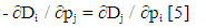
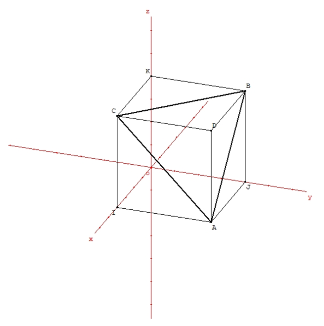
The first tractable example is interesting because … the demands are not linear. One supposes a density of utility which is areal, homogeneously distributed on the external facets of the cube u_i = 1 (this density is equal to 1/3) (figure 2). The formulas for the demands depend of inequalities such as p₁ < p₂ < p₃ etc.

Figure 2. In the first tractable example the density is areal, homogeneous and distributed on the external facets of the cube. These facets are stripped on the figure

For instance, if p₁ ≤ p₂ ≤ p₃:

D₁ = 1/3 [1 + p₁²/2 – p₃²/2 – p₁ p₂ + p₂ p₃ – 2p₁ + p₂ + p₃]

D₂ = 1/3 [1 – p₁²/2 – p₃²/2 + p₁ p₃ + p₁ -2p₂ + p₃]

D₃ = 1/3 [1 + p₃² + p₁ p₂- p₁ p₃ – p₂ p₃ + p₁ + p₂ -2p₃]

Of course, the Nash equilibrium is on the diagonal (0, 0, 0) (1, 1, 1) and there are different formulas for p₁ < ½ and p₁ > ½, for instance. The Nash equilibrium is at (½, ½, ½) and the profits are equal to 1/6. But there is a discontinuity of the tangent to the reaction function, at the equilibrium point. One cannot define the determinant of the Jacobian. However, the particular demonstration of the previous paragraph allows to state that if the firm E₁ adds k to the utilities u₁ (u₁ → u₁ + k, k > 0), its profit P₁ increases.

The second tractable example is simpler, since the demands are linear. The Jacobian is defined and is negative (the equilibrium is stable for small variations of the prices). The second derivatives of the demands are equal to 0. One supposes that the density is linear, homogeneously distributed and on the second bisector in each external facet u_i = 1 (density equal to 1 /3√2). The density is shown on the figure 3.

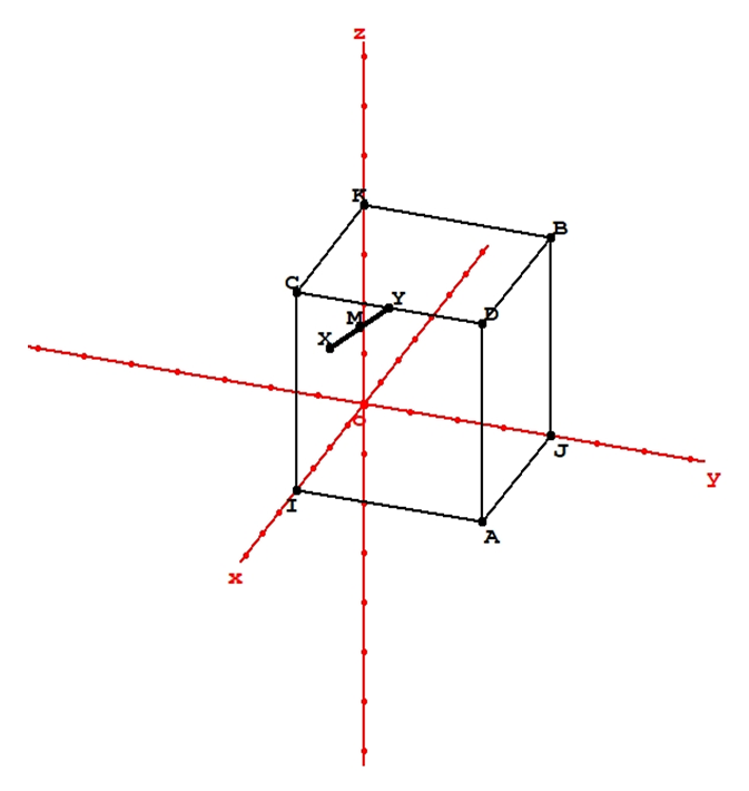
Figure 3. The density in the case of the second tractable example is shown. It is linear, homogeneous and distributed on the second bisectors in the external facets of the cube

The demands are:

D₁ = 1/3 [1 -2p₁ + p₂ + p₃]

D₂ = 1/3 [1 + p₁ -2p₂ + p₃]

D₃ = 1/3 [1 + p₁ + p₂ -2p₃]

The Nash equilibrium corresponds to p₁ = p₂ = p₃ = ½ and P₁ = P₂ = P₃ = 1/6. To study disruption in this case, one can suppose that E₁ increases all the utilities of 1. The demands become:

D’₁ = 1/3 [3 -2p₁ + p₂ + p₃]

D’₂ = 1/3 [p₁ -2p₂ + p₃]

D’₃ = 1/3 [p₁ + p₂ -2p₃]

(provided that for p₁, p₂, p₃ all the D_i are positive).

One checks that for (1, 0, 0) all the demands are 1/3. It is extremely advantageous for E₁, since its price is high (compared to the two other prices) and it keeps the consumers in its “garden” (that is to say the consumers preferring the product sold by E₁).

One easily calculates the profits at the Nash equilibrium p’₁₀ = 9/10, p’₂₀ = p’₃₀ = 3/10 (in accordance with the model, p₂ and p₃ decrease): P’₁ = 54/100 (which is more than 1/6) and P’₂ = P’₃ = 3/50 (which is less than 1/6). In accordance with the model, the profit P₁ increases and the profits P₂ and P₃ decrease.

One has to check that the Nash equilibrium is “inside the formulas” (D_i ≥ 0). It is not necessary in the case of that example because the demands are linear. Since ∂P_i / ∂p_i = D_i + p_i ∂D_i / ∂p_i = 0, ∂D_i / ∂p_i being a negative coefficient (the demand D_i is linear), D_i ≥ 0.

The second tractable example is resumed later in the paper. One considers a value of k which is ½, not 1, to be “inside the formulas”. The game is with two players, since one considers a “buy and manage” and a “buy and close down”.

6. About the Possibilities of the Model Used

A goal of this paper is to show the possibilities of the model used (Bertrand competition, the demands being deduced from the consumers ‘utilities).

The model can be used to study the profitability of a merger, when the asset which is bought is closed, to discriminate between non differentiating innovation and differentiating innovation, and study the effects of cannibalization:

Profitability of buy and close down.

This kind of operation, to buy an asset and to close down it, which is supposed to be profitable (otherwise the managers would not have decided it) seems rare. Indeed, it is discrete, because the Opinion disapproves any destruction of means of production. In France, several years ago, the firm UPM (United Paper Mills) decided to close a site where paper was produced, in a village (Docelles). During a night, members of the staff destroyed the machine. It was made by night, not because it was illegal, but because it was scandalous. The destroyed machine could not be resold, and the firm lost money. But another unit of the same firm should benefit from higher prices. This compensates and besides the loss of money. It is the same calculation than in the case of “buy and close down”.

The topic is interesting for several reasons:

- The question of the regulator’s reaction is posed. He could disapprove this operation, which shrinks competition. But his opposition is easy to circumvent. It is easy to not invest in a branch, or to not invest enough, and some day one has to close it.

- The profitability of an operation “buy and close down” is obviously a sign of saturated market. In case of Bertrand competition, a merger is always profitable (given some conditions). The profitability of a merger cannot be the sign of a saturated market. But the profitability of an operation “buy and close down” implies a strong strategic effect, because of less competition. It is explained by the saturation of a market. Two causes (when a market is saturated) are possible: (1) a competitor creates low utility for consumers, is obliged to choose a low price and “steals” customers from the other competitors (2) the products are not enough differentiated, that is to say the Bertrand paradox applies. The model used allows to present tractable models of the two kinds [4].

- When the “buy and close down” is profitable, it is a reason more to choose the merger (“buy and manage”), because there is an insurance. Often to “integrate” the bought firm in the buying firm is difficult [7]. Quarrels between the two teams of managers can raise. If the “buy and close down” is profitable, it is easy to make pressure on the team of managers of the bought firm (“if you do not cooperate, we can close down the asset, it will remain profitable”). Therefore, the profitability of the “buy and close down”, if it exists, incites to merge.

Non differentiating innovation and differentiating innovation.

There is non differentiating innovation when an innovation is beneficial to all the competitors. In the model, all the utilities u_i become u_i + k (k> 0). If at the start there is product differentiation, the “gardens” correspond to the utility 1 + k. The profits increase. But there is a drawback: when the increase of all the utilities is the same, there is less product differentiation. An easy calculation which is not set out in this paper, shows this: non differentiating innovation can trigger a kind of saturated market (at the start, a “buy an close down” is not profitable, then after non differentiating innovation it becomes profitable).

Let us give an “example of non-differentiating innovation. The dressmaker Karl Lagerfeld (1939 – 2019) made his career in Paris and was notorious. He worked in many firms which were in competition: in high fashion (Chanel, Fendi and his own firm), in ready to wear (Chloe, H&M) and even in sale on line (NetaPorter). Thanks to his talent, he brought innovation in several firms in competition. Therefore, the consumers ‘utilities increased. The consequence was that the profits of the firms in which he worked increased (and himself won more money). This seems to be a digression but perhaps is not. The author has stated in a paper that there is a production function of the modern artist [8]. An artist has to be visible (participating in galas, events, having a humanitarian activity, appearing in medias … to have an “image”) and to be creative (in his works). The artist’s gain is an increasing function of the two factors (visibility and creativity). In this sense, Karl Lagerfeld was really a moderncartist. He wqas an entrepreneur in visibility and creativity. His prolific activity is accurately depicted in the book “Karl Lagerfeld de A à Z” [9].

At the opposite, differentiating innovation (disruption) is beneficial to a single firm, the disruptive firm. But a disruptive firm should not “buy and close down” a competitor. It is to shrink competition thanks to a means that the regulator could refuse.

In his book “The innovator’s dilemma”, Christensen has explained that a firm the market of which is threatened by innovating competitors will react by protecting its market, aiming at keeping its customers thanks to an upgrade of its product. It is risky because some day the new products could replace its own [10]. Of course, there is the temptation to buy and close down the innovating firm which is a threat. The threatening firm could also be bought then its development is slowed. A famous example is Instagram bought by Facebook. It has been said that years later, Instagram could have become a real leader (as Facebook), but it has been bought by Facebook. This is made possible by the fact that it is difficult to value a start-up (in the fields of Information Technologies or bio-engineering, for instance). Examples are given in the article “Antitrust and innovation: welcoming and protecting disruption” [11].

Recently fears have appeared that the regulation in the USA, could slacken. This fear is expressed in the Philippon’s book “The great reversal: how America has given up on free markets” [12].

All this shows that the profitability of operations of “buy and close down” is an interesting topic. Since disruption is wished and welcomed, one fears an incumbent which “buys and closes down” a small, innovating firm which threats its market or its product.

Effects of cannibalization.

The model can be used to study the effects of cannibalization. One gives a tractable example in the following chapter.

7. A Tractable Example on Disruption

There are often portfolios of brands in many fields: technology, fashion (clothes, leather goods, jewelry …) or medias. These brands are often in competition. These portfolios of brands in competition pose puzzling questions. Is it in the interest of the owner to choose a disruptive strategy for one of his firms, given that it will harm the other very much? Is it not in his interest to choose disruption for one of his firms and close down another? These questions could be interesting for the regulator, too. Possibly, the regulator could disagree, if the owner of several firms in competition buys a firm with the intention of not developing it, perhaps of closing down it (to develop another firm he owns).

One can use the second tractable example set out in the paper to illustrate the effect of cannibalization.

The disruption can be achieved in three ways:

- At the start, there is equilibrium with three firms, “monopolistic competition”. One calls this game E (as equilibrium).

- At the start, the disruptive firm E₁ has bought E₃ and will keep it. One calls this game BM (as Buy and Manage).

- At the start, the disruptive firm E₁ has bought E₃ and will close down it. One calls this game BC (as Buy and Close down).

The calculations show that E is less profitable than BC, which is less profitable than BM. How to explain that BC is less profitable than BM? In case of BC, the disruptive firm does not benefit from the profit of E₃, but there is no cannibalization. At the opposite, in case of BM, the disruptive firm E₁ benefits from the profit of E₃, but there is cannibalization (that is to say, E₃ “steals” customers from E₁, and the margin is less, because p₃ < p₁).

The calculations are needed to know what is more profitable (BM or BC).

One can put it in other words. Consider BM, after disruption. One passes to BC by closing E₃ (p₃ = 1), then the two prices p₁ and p₂ change and the two profits P₁ and P₂ change, also. What happens when p₃ becomes equal to 1? There are three kinds of customers of E₃: (1) those choosing E₁. It is the effect “end of cannibalization”, since these customers will allow the margin p₁ instead of p₃ (and p₁ > p₃) (2) those choosing E₂ who are customers lost for E₁ and (3) those choosing no purchase, who are also customers lost for E₁. The demand for E₁ has decreased (D₁ is less after p₃ → 1 than D₁ + D₃ before). After, there are changes of p₁ and p₂, and one does not know the change of D₁. The calculations show that the demand D₁ is less, after the close down. This explains that the profit is less. And this, notwithstanding the cannibalization which no more exists. The outcome is “reassuring” for the regulator. A disruptive firm should not buy a competitor then close down it. It should buy it and keep it. Notice that one has only examined a particular case.

This question is interesting, since the disruptive firm benefits from high margins during a first period, only. There are three periods. During the first one the disruptive firm has a behavior described by speed and brand. The goal is growth. It has to make its product well known and attractive for customers. The high margins do not last a long time because during the second and third period there are entries and imitators [10]. The two last periods are necessary to make the prices of the new products lower, which is a condition of disruption according to Christensen (the products are “affordable and accessible”). During the first period, there are priorities and other goals like reduction of the costs or upgrading the distribution of the product, are neglected. And in this first period, the disruptive firm could be interested in buying a competitor, if it allows more profit.

8. Conclusions

One has modelled “monopolistic competition”, or product differentiation, thanks to a method which is presented in the paper: Bertrand competition, the demands being deduced from the consumers’ utilities. The mathematical properties of the equilibrium, the existence of which is demonstrated, correspond to the characteristics of product differentiation: all the consumers buy a product, the competitors benefit from a “garden” (a set of customers easily kept) and the profits are sufficient. Disruption is defined: the “garden” of the disruptive firm has a utility which is more than the utilities of the “gardens” of the other competitors. One demonstrates that the profit of a firm which disrupts, increases.

A goal of the paper is to explore the possibilities of the method presented. This method allows to study these topics: the profitability of mergers when the asset which is bought is closed down, the difference between non differentiating innovation and differentiating innovation (disruption) and the effects of cannibalization.

Tractable examples are set out, which allow to illustrate how the method can be used. For instance, a tractable example brings an answer to the question: What it the most profitable for a disruptive firm: to “buy and manage” a competitor, to “buy and close down” it or to make no purchase? This question implies to study the effects of cannibalization.

Could this method be upgraded? One can deal with this question considering three aspects:

- The choice of three players. It is chosen to simplify. It would be easy to generalize the game to n players.

- Neglecting the costs. Let us recall the difference between “disruptive innovation” and “efficient innovation” according to Christensen. We have already quoted the definition of “disruptive innovation”. The efficient innovation is an innovation which does not concern the product, but triggers a decrease of the costs [13]. Since the goal of this paper is to study disruptive innovation, to neglect the costs is without consequences.

- The problem of moral obsolescence. It can be understood thanks to a cognitive bias, sometimes called the “dolphin bias”. It has been described, among other cognitive biases, by Nassim Taleb [14]. It concerns an inquiry on these questions: “How much money do you want to give to save dolphins?” and “How much money do you want to give to save kids from some illness?”. The results are not the same if the questions are posed separately or simultaneously. If the questions are separately posed the answers could be 50 dollars (first question) and 30 dollars (second question). If the questions are simultaneously posed, the order is reverse: 30 dollars (first question) and 50 dollars (second question). In other words, evaluation of something depends on information. When the consumers having chosen the old product are informed on the new product, their evaluation of the utility of the old product decreases (in particular when the usage implies networks). In the model used on the paper, in case of disruption one could change u₁ into u₁ + k (k>0), E₁ being the disruptive firm, u₂ into u₂ – k₂ (k₂ > 0) and u₃ into u₃ – k₃ (k₃ > 0), E₂ and E₃ being the other competitors. This means that the profit P₁ would increase more, and the profits P₂ and P₃ decrease more.

The model used seems interesting, in particular, because it provides a criterium for saturated markets (the profitability of “buy and close down”). Perhaps practical applications should be possible. Market studies provide a cloud of points representing the utilities of the consumers. It corresponds approximately to an analytical function, or not. If not, a computer could be used to find the Nash equilibrium (provided that it exists and is unique). After, to calculate if the “buy and close down” is profitable, or not, should be feasible. If the “buy and close down” is profitable, it is a criterium indicating that the market is saturated.

Note

1. For Christensen, «disruptive innovation» allows products which are more useful and more accessible. It is the motor of economic growth. For instance, the progress in computer technology allowed mainframe computers, then personal computers, and finally smartphones.