-
Paper Information
- Paper Submission
-
Journal Information
- About This Journal
- Editorial Board
- Current Issue
- Archive
- Author Guidelines
- Contact Us
Journal of Game Theory
p-ISSN: 2325-0046 e-ISSN: 2325-0054
2020; 9(2): 25-31
doi:10.5923/j.jgt.20200902.01
Received: Sep. 21, 2020; Accepted: Oct. 20, 2020; Published: Oct. 28, 2020

A Comprehensive Review of Solution Methods and Techniques for Solving Games in Game Theory
 Abstract
 Reference
 Full-Text PDF
 Full-text HTML
Issah Musah, Douglas Kwasi Boah, Baba Seidu
Department of Mathematics, C. K. Tedam University of Technology and Applied Sciences, Navrongo, Ghana
Correspondence to: Douglas Kwasi Boah, Department of Mathematics, C. K. Tedam University of Technology and Applied Sciences, Navrongo, Ghana.
| Email: |  |
Copyright © 2020 The Author(s). Published by Scientific & Academic Publishing.
This work is licensed under the Creative Commons Attribution International License (CC BY).
http://creativecommons.org/licenses/by/4.0/

This paper presents a comprehensive review of solution methods and techniques usually employed in game theory to solve games with the view of demystifying and making them easy to understand. Specifically, the solution methods and techniques discussed are Nash Equilibrium Method; Pareto Optimality Technique; Shapley Values Technique; Maximin-Minimax Method; Dominance Method; Arithmetic Method; Matrix Method; Graphical Method and Linear Programming Method. The study has contributed significantly to knowledge by successfully filling or narrowing the knowledge or research gap of insufficient literature on reviews of solution methods and techniques usually employed to analyze or solve games in game theory.
Keywords: Games, Solution Methods, Techniques, Game Theory, Strategies, Payoffs, Value of a Game
Cite this paper: Issah Musah, Douglas Kwasi Boah, Baba Seidu, A Comprehensive Review of Solution Methods and Techniques for Solving Games in Game Theory, Journal of Game Theory, Vol. 9 No. 2, 2020, pp. 25-31. doi: 10.5923/j.jgt.20200902.01.
1. Introduction
- Singh [1] defined a game as a competitive situation among N persons or groups called players conducted under a prescribed set of rules with known payoffs. The rules define the elementary activities or moves of the game. According to Bhuiyan [2], the rules of a game are defined by the players, actions and outcomes. The decision makers of a game are the players. All possible moves that a player can make are called actions. One of the given possible actions of each competitor or player is referred to as a strategy. A pure strategy is deterministically selected or chosen by a player from his/her available strategies. On the other hand, a mixed strategy is one randomly chosen or picked from amongst pure strategies with allocated likelihoods. Expected gain a player gets when all the other players have picked or chosen their possible actions or strategies and the game is over is referred to as utility or payoff. A set of obtained results emanating from the possible moves when the game is played out is called outcome. Darkwah and Bashiru [3] stated that, a combination of strategies that comprises the optimal or best response for each of the players in a game is called equilibrium. Morrow [4] presented that, there are mainly two ways to represent a game namely the normal form (which is simply a matrix that describes the strategies and payoffs of the game) and the extensive form (which is a tree-like form or structure. However, there are games that require richer representation such as infinite repeated games. According to Shoham and Leyton-Brown [5], to represent such games, we go beyond the normal and extensive forms. Usually, games are categorized according to their characteristics or features. Some common types of games are as follows:(i) Coalitional and non-coalitional games: A coalitional game is one in which players agree to employ mutual or reciprocal strategies and gain higher benefits. An example of non-coalitional game is Prisoner’s dilemma game. (ii) Prisoner’s dilemma game: This is a situation whereby two suspected criminals are taken custody by the police and charged. In addition, information available to the police is insufficient to prove that they are guilty of the crime, unless one confesses or both of them confess. Now, each one of them can either admit the crime hoping to be given a lighter punishment or decide not to talk. Consequently, the police interrogate or question the suspected criminals in separate rooms and offer them deals. If both of them refuse to talk, then each one of them will be charged with minor crime and given say one-month jail term. Again, if both of them confess, each one of them will be given say a six-month jail term. Moreover, assuming one confesses and the other does not do that, the confessor is liberated while the other one given say, a nine-month jail term. In fact, the game is a tactical one. The players of the game pick or select their possible actions or strategies at the same time only once, and then the game is completed. (iii) Zero-sum game: Zero-sum games are the mathematical representation of conflicting situations according to Washburn [6] and that in those games, the total of gains and losses is equal to zero.(iv) Two-person zero-sum game: According to Hillier and Lieberman [7], it is a competitive situation involving exactly two competitors whereby one of them wins what the other loses.(v) Nonzero-sum game: This is one whereby the total utility for every stage or outcome is not zero. Nonzero-sum games are categorized into two distinct types namely ‘constant-sum games’ and ‘variable-sum games’. The former is one whereby the total utility for each outcome is a fixed value whereas the latter is one whereby the sum of all the utilities for each outcome gives different values. According to Kumar and Reddy [8], game theory is concerned with uncertain decisions comprising two or more opposing and intelligent agents or people whereby each one of them aims to outwit the other (s). Dixit and Skeath [9] defined game theory as a discipline that studies decision making of interactive entities and asserted that strategic thinking is perhaps the most recognized essence of game theory. Shoham and Leyton-Brown [5] stated that, game theory presents a technical analysis of strategic interactions which according to Geckil and Anderson [10] are concerned with the interaction of decision makers in the game. In fact, game theory provides a platform which can be used to formulate, analyze and understand different strategic situations.This paper presents a comprehensive review of solution methods and techniques usually employed in game theory to solve games with the view of demystifying and making them easy to understand.
2. Literature Review
- The first information about game theory was set forth by James Waldegrave in 1713. In his letter, he presented a solution to a two-person card game with mixed strategies. In 1921, Emile Borel suggested a formal way of handling game theory. In 1928, his suggestion was advanced by John Von Neumann in his published paper that served as the foundation of a two-person zero-sum game. In 1944, Oskar Morgenstern and John Von Neumann presented a book titled ‘The Theory of Games and Economic Behaviour’. That move was believed by many to give rise to game theory as an area of research or learning. In 1950s, John Nash, Harold Kuhn, John Harsanyi etc. developed game theory intensely. According to Von Stengel [11], John Nash advanced the tools and ideas of game theory proposing the universal ‘cooperative bargaining and non-cooperative theories’. He brought forth what is presently termed the ‘Nash equilibrium’ of a tactical game in 1951 by establishing that every finite game at all times has an equilibrium point, at which every competitor selects moves which are paramount for them being fully aware of the selections or picks of his/her competitors or challengers. Game theory was expanded theoretically and used to solve warlike, political and philosophical issues in the 1950s and 1960s. The concept of game theory has since received much attention. A number of papers in the theory and applications of queuing theory have been reported in the literature. Moulin and Vial [12] proposed a class of games with special payoff structure called strategic zero-sum games. Ponssard and Sorin [13] discussed zero-sum games with incomplete information. McCabe et al [14] studied a three-person matching pennies game. Athey [15] studied incomplete information games and proposed a restriction called single crossing condition for those games. Chang and Marcus [16] studied two-person zero-sum game taking into consideration optimal equilibrium game value and then analysis of error bounds. Maeda [17] considered games that have fuzzy payoffs. Edmonds and Pruhs [18] proposed a randomized algorithm taking into consideration cake cutting algorithm. Al-Tamimi et al [19] discussed Q-learning designs for the zero-sum game and used a model-free approach to obtain a solution for the game. Larsson et al [20] studied signal processing and communications in a game theoretic way. Li and Cruz [21] used a zero-sum game model with an asymmetrical structure to study deception. Singh [1] presented optimal solution strategy for games. Duersch et al [22] obtained Nash equilibrium for the 2-player symmetric game. Perea and Puerto [23] used game theory approach in network security. They examined a game between a network operator and attackers. Procaccia [24] discussed a cake cutting game describing it as a powerful tool to divide heterogeneous goods and resources. Spyridopoulos [25] studied a problem of cyber-attacks using a zero-sum one-shot game theoretic model. Bell et al [26] proposed a game theoretic approach for modelling degradable transport networks. Bensoussan et al [27] studied non-zero-sum stochastic differential game and modelled the performance of two insurance companies. Gensbittel [28] studied zero-sum incomplete information games. Grauberger and Kimms [29] computed Nash equilibrium points for network revenue management games. Singh and Hemachandra [30] presented Nash equilibrium for stochastic games with independent state processes. Marlow and Peart [31] studied soil acidification describing a zero-sum game between a sugar maple and American beach. Boah et al [32] used game theory to analyse the levels of patronage two radio stations in Kumasi, Ghana. Daskalakis et al [33] proposed a no-regret algorithm capable of achieving regret when applied against an adversary. Bockova et al [34] applied game theory to project management. Farooqui and Niazi [35] reviewed game theory models for communication between agents. Gryzl et al [36] presented how game theory can be employed to manage conflict in a construction contract. Stankova et al [37] presented how treatment of cancer can be optimized using game theory. Padarian et al [38] employed game theory to interpret a ‘digital soil mapping model’. To the best of our knowledge and from literature, reviews of solution methods and techniques for solving games in game theory are not sufficient and comprehensive enough. The study was therefore intended to fill or narrow that knowledge or research gap.
3. Main Work
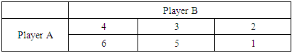
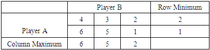
- The solution methods and techniques usually employed to solve games in game theory are as discussed below:(i) Nash Equilibrium MethodNash equilibrium is a solution method of a ‘non-cooperative’ game concerning two or more competitors in which each competitor is assumed to have knowledge of the equilibrium or stability tactics of the other competitors, and no competitor has whatsoever to gain by varying only his/her individual tactic. If each competitor has selected a tactic or strategy, and no competitor can profit by varying tactics while the other competitors hold onto their tactics or strategies, then the present chosen tactics or strategies and their analogous utilities constitute ‘Nash equilibrium’. For example, Daniela and Derrick will be in ‘Nash equilibrium’ if Daniela makes the finest decision possible, taking into account Derrick’s decision which remains constant, and Derrick also makes the finest decision possible, taking into account Daniela's decision which remains constant. Similarly, a set of competitors will be in ‘Nash equilibrium’ if every single one makes the finest decision possible, taking into consideration the decisions of the other competitors in the contest which remain constant. According to Nash, “there is Nash equilibrium for every finite game”. Experts in game theory utilize the concept of ‘Nash equilibrium’ to examine the consequence of tactical collaboration of a number of decision makers. Ever since the concept of ‘Nash equilibrium’ was developed, experts in the field of game theory have revealed that, it creates misrepresentative forecasts or predictions in some situations according to Nash Jr [39].(ii) Pareto Optimality TechniquePareto optimality was first introduced by Vilfredo Pareto according to Yeung and Petrosjan [40]. In a Pareto optimal game, there exists a strategy or tactic that increases a player’s gain without harming others. For example, when an economy is perfectly competitive, then it is Pareto optimal. This is because no changes in the economy can improve the gain of one person and worsen the gain of another simultaneously. (iii) Shapley Values TechniqueAccording to Shapley [41], this is a solution technique or concept used in cooperative game theory. It assigns a distribution to all the players in a game. The distribution is unique and the value of the game depends on some desired abstract characteristics. In simple words, Shapley value assigns credits among a group of cooperating players. For example, let us assume that there are three red, blue and green players and the red player cooperates more than the blue and green players. Now, if the objective or goal is to form pairs and then assign credits to them, each pair must have a red player as it cooperates more than the other two. Therefore, there can be two possible pairs namely red player-blue player and red player-green player. The red player cooperates more and for that matter will get more profit than the blue player in the first pair. Similarly, the red player will get more profit than the green player in the second pair.(iv) Maximin-Minimax MethodThis method is used in both games with pure and mixed strategies. In the case of a game with pure strategies, the exploiting player reaches his/her optimum strategy on the basis of the maximin principle. Conversely, the diminishing player reaches his/her optimum strategy on the basis of the minimax principle. The difference between pure and mixed strategy games is that, pure strategy games possess saddle points whereas mixed strategy games do not. According to Washburn [42], a saddle point is a point at which ‘the minimum of column maximum’ is equal to ‘the maximum of row minimum’. If both the ‘maximin’ and ‘minimax’ values are zero, such a game is referred to as a fair game. When both the maximin and minimax values are equal but not zero, then the game is referred to as strictly determinable.
|
|
 by first of all deleting Row 3 which is dominated by Row 2 to obtain
  and finally deleting Column 3 which is dominated by Column 1 to obtain
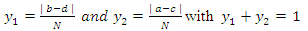
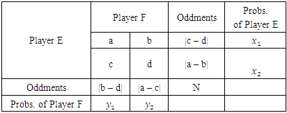
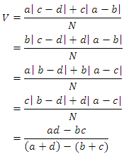
  . (vi) Arithmetic MethodThis is a method that provides a comprehensible approach for obtaining optimal strategies for every player in a 2
  2 pay-off matrix with no saddle point. If the payoff matrix is lengthier than 2
  2, then the dominance method would be employed and finally the algebraic procedure to help obtain the optimal strategies and also the value of the game. This method or procedure is also called the Method of the Oddments according to Piyush [43].
|
 •
•  Steps (i) to (v) therefore yield the resulting matrix as given in Table 4.
|
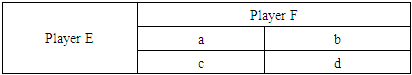
 (vii) Matrix MethodThis method provides a way of finding optimal strategies for players in 2
  2 games. Given a payoff matrix
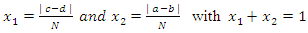
 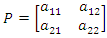 , the best strategies for both players A and B could be obtained in addition to the value of the game for player A.Player
  optimal strategies
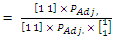
 Player
  optimal strategies
 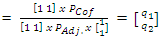 The value of the game, V= (Player
  optimal strategies) × (Payoff matrix, P) × (Player
  optimal strategies)That is,
 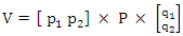 where
where  and
and 
 represent the probabilities of players A and B’s optimal strategies respectively.
  and
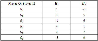
and  are the adjoint and cofactor of the payoff matrix respectively as presented by Piyush [43].(viii) Graphical MethodThe graphical method is used to solve games with no saddle points. It is restricted to 2 x m or n x 2 matrix games only according to Kumar and Reddy [8]. To illustrate the graphical method, let us consider the payoff matrix given in Table 5.
|
|
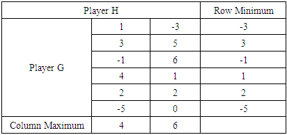
 Minimax, the game has no saddle point. Therefore, the problem is handled using the graphical method as follows:
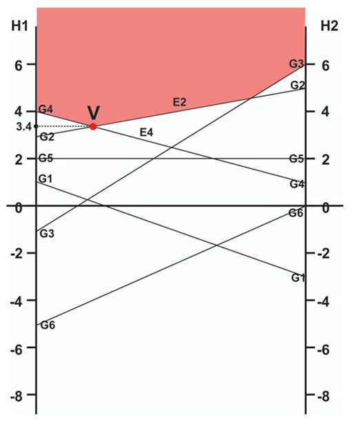 | Figure 1. Graph of the Payoff Matrix for Players G and H |
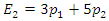 | (1) |
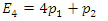 | (2) |
 | (3) |
 into equation (3), we have
 yielding
  and
and  Substituting the values of
  into equation (1), we obtain
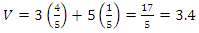 Therefore, the value of the game, V to Player G is 3.4 as already indicated.(ix) Linear Programming MethodLinear programming (LP), also called linear optimization, is a method used to achieve the best outcome for an objective (such as maximum profit or minimum cost or other measures of effectiveness) in a mathematical model whose requirements are represented by linear relationships according to Williams [44]. According to Sharma [45], the two-person zero-sum games can be solved by LP. The major advantage of using linear programming technique is that, it helps to handle mixed-strategy games of higher dimension payoff matrix. To illustrate the transformation of a game problem to an LP problem, let us consider a payoff matrix of size m x n. Let
  be the entry in the
  row and
  column of the game’s payoff matrix, and let
  be the probabilities of m strategies
  for player A. Then, the expected gains for Player A, for each of Player B’s strategies will be:
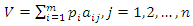 The aim of player A is to select a set of strategies with probability
  on any play of game such that he can maximize his minimum expected gains. Now to obtain values of probability
  the value of the game to player A for all strategies by player B must be at least equal to V. Thus to maximize the minimum expected gains, it is necessary that:
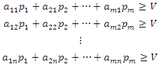 where
where 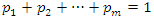 and
and  for all
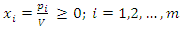
  Dividing both sides of the m inequalities and equation by V, the division is valid as long as
  In case,
  the direction of inequality constraints is reversed. If
  the division becomes meaningless. In this case, a constant can be added to each of the entries of the matrix, ensuring that the value of the game (V) for the revised or updated matrix becomes more than zero. After the optimal solution is obtained, the actual value of the game is found by deducting the same constant. Let
 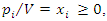 we then have
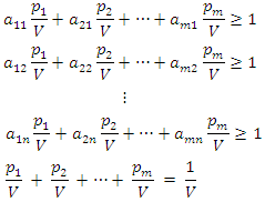 Since the objective of player A is to maximize the value of the game, V, which is equivalent to minimizing
  , the resulting linear programming problem, can be stated as:
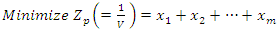 Subject to the constraints:
 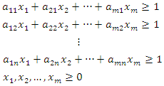 | (4) |
 Similarly, player B has a similar problem with the inequalities of the constraints reversed, i.e. minimize the expected losses. Since minimizing V is equivalent maximizing
  , the resulting linear programming problem can be stated as:
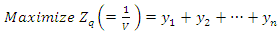 Subject to the constraints:
 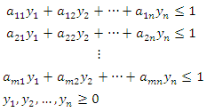 | (5) |
4. Conclusions
- In this paper, a comprehensive review of solution methods and techniques usually employed in game theory to solve games has been presented with the view of demystifying and making them easy to understand. Specifically, the solution methods and techniques discussed are Nash Equilibrium Method; Pareto Optimality Technique; Shapley Values Technique; Maximin-Minimax Method; Dominance Method; Arithmetic Method; Matrix Method; Graphical Method and Linear Programming Method. The study has contributed significantly to knowledge by filling or narrowing the knowledge or research gap of insufficient literature on reviews of solution methods and techniques for solving games in game theory.