1. Introduction

In the literature has been widely discussed how different information settings influence the decisions of banks and investors in the credit market. Mostly, we have a situation where the players do not have complete information about the details of interaction. Usually, this takes place when the lender is uncertain of the borrower’s risk type. Because of different probability distributions of the unknown parameter games of asymmetric information are played.

In project funding a game of asymmetric information is to be considered when only the borrower knows the real risk of the project he chooses but the lender does not. Typically, the assumption of a discrete probability distribution on two points for the cash flows generated by risky projects leads to the well-known positive signalling results. If so, from the lender’s side appropriately defined financial measures are helpful signals for revealing projects’ risks with a high degree of certainty.

However, less well-known is how signalling works when the cash flows of uncertain projects are not modelled by a two point probability distribution. Using the debt-to-equity ratio, chosen by the borrower before receiving a lender’s loan to finance a project, as measure we deal with the question whether a positive signalling result can still be confirmed when probability distributions with continuous densities for the cash flows are assumed. More precisely, in a borrower-lender game without cash flows’ restrictions due to discrete distributions on two points it is questioned whether a separating perfect Bayesian equilibrium (PBE) exists.

Before proving a non-positive result, at first, a short justification for our analysis is given. For that purpose the assumptions of three pioneered works are sketched briefly (i) Ross [1] presumes high debt levels as signals for high quality investments. The firm’s probability distributions of projects’ returns are different by first-order stochastic dominance. In the paper, the projects are ranked according to second-order stochastic dominance (ssd) (see [2]) characterized by mean-preserving spreads (mps), (ii) Bester [3] assumes the loan level as signal for the probability of default. The lender is imperfectly informed about the investor’s risk type. By using a discrete probability distribution on two points, the project’s outcome is either a zero cash flow if the project fails or a positive cash flow if the project succeeds. In the paper, a continuum of outcomes is assumed. The size of the projects is exogenously given by an initial outlay. By choosing the loan level, the investor also decides on the level of equity, he is willing to commit to the project, and (iii) as well, loan size as signal of projects’ risks is supposed by Milde/Riley [4]. The probability distributions of projects’ returns are different by ssd. Just as Bester, Milde/Riley assume that the return depend on both a quality parameter known only the loan applicant and the loan size. There is no upper bound for the loan size choice. Assuming limited liability, the paper deals with the question whether the debt-to-equity ratio is a signal for revealing projects’ risks.

The remainder proceeds as follows. Section 2 is divided in two subsections. Firstly, we define a simple borrower-lender game (see 2.1). Secondly, for solving the game the PBE is used (see 2.2). Section 3 concludes. The main result (the non-existence of a separating PBE) is proven indirectly. The proofs are collected in an Appendix.

2. The Setting

A firm loans a credit to fund a one period project with uncertain cash flows. There are two types of risky projects. Increasing risk is expressed by mps of the projects’ cash flows. The type is private knowledge of the firm. The bank only knows that have low risk (class 1) and have high risk (class 2). It is unknown which project is funded after receiving a loan. The stochastic of the types is common knowledge. The risk-free interest rate is zero.

Independent of the type of risk running a project requires financial funds . The loan volume 1 (the debt-to-equity ratio) is to be chosen by the firm. A loan of at least and is assumed (Note that only a ratio bigger than 1 implies project funding is risky for the bank). Depending on the loan amount chosen by the firm for any possible loan the bank decides on the extra charge to the risk less interest rate by choosing schemes of loan offerings (claims) . The difference is covered by the equity of the owners of the firm. The players are risk-neutral.

Now, we question whether a debt-to-equity ratio is a signal for reducing the bank’s uncertainty of the firm’s risk type. The idea of the firm’s risk self-selection is the following: the bank unable to identify the risk of a project chosen by the firm offers for revealing the firm’s hidden risk some different loan contracts to conclude from the ratio chosen by the firm with certainty what the firm’s risk type will be.

2.1. The Borrower-Lender Game

Before starting the analysis, foresighted we summarize briefly. By assuming (i) a continuous projects’ cash flow probability distribution, (ii) a projects’ ranking by ssd, and (iii) limited borrowers’ liability a game is analyzed in which, how we show, assumption (i) is decisive for the type of the PBE. The sequence of players’ moves is depicted in figure 1.

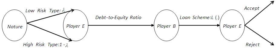Figure 1. Players’ sequence of moves

The following assumptions and notations are taken: (i) Firm E and bank B are the players. Player E chooses either a project of type or type . Both projects require the same initial amount . (ii) The projects’ cash flows are uncertain. The random variable is given by the distribution and the density with for all and else. (iii) Both distributions have the same expected value . The -project is riskier than the -project, which is expressed by ssd. The stochastic of the projects’ types is common knowledge. (iv) Player B does not know player E’s type. Player E chooses the debt-to-equity ratio (the loan face value) . Player B chooses (supplies) a loan scheme (the claim) for any .

The cash flows are calculated as follows: if a loan with a face value 1 and a corresponding claim are accepted by player E, then player E’s cash flow is given by if 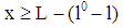is valid (case of non-insolvency). Otherwise, player E’s cash flow is given by 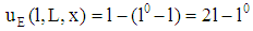(case of insolvency). At player B’s cash flow is given by 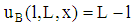if is valid and else.

Remark 1: (i) The analysis is limited to project funding with limited liability. In case of insolvency, the bank’s rights are restricted to the cash flows generated by the firm’s (the owners of the firm) equity. (ii) For keeping the analysis simple a risk less interest rate is assumed, whereat is valid. (iii) Running a project requires a strictly positive minimum debt-to-equity ratio. More than the half of the total investment sum of the project to be a loan is required. Otherwise, independent of the real risk type a project is certain for the bank. Due to the liable equity must be at least as large as the bank’s claim for loans.

2.2. The Game Theoretic Analysis

To analyze the borrower-lender game the PBE is used. It is described by a pair with . Here, and denote the loan size chosen by the firm depending on its type. The bank’s system of beliefs (i.e., a probability assessment) with respect to the firm’s risk types is denoted by . For a chosen ratio given by the requested loan par value 1 the bank’s system of beliefs is given by (i.e., the bank’s subjective probability that the chosen project is of type ) and (i.e., the bank‘s subjective probability that the chosen project is of type ).

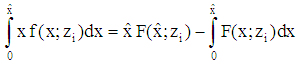
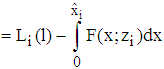
For solving the game, at first, we determine the type specific expected payoffs of the players if the firm accepts the bank’s claim with a par value f. Denotes the boundary of insolvency we get (1) 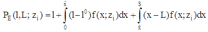and (2) 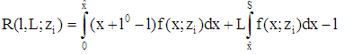. Due to the beliefs the bank’s type specific expected payoff is given by (3) 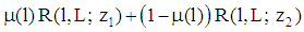. Denotes 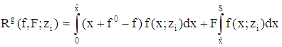the bank’s type-specific (conditional) expected payoff, then the bank’s claim supply for a par value 1 is implicitly given by (4) .

Remark 2 We assume perfect competition for the firms within a homogeneous group of banks. A loan contract satisfying (4) includes the minimum claim of a risk neutral bank with respect to a loan with par value 1 in a perceived situation . More precisely, in the game the bank always offers the best possible contract to the firm since the lowest possible charge on the risk free interest rate is chosen by the bank.

Next, we prove the main result. The basic idea is illustrated in figure 2 below. Referring to the Appendix first of all a few remarks about some properties of the firm’s indifference curves (see remark 3 and remark 4) will be made briefly: (i) The slope of a type i-firm curve at is given by (5) 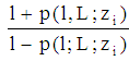. (Note: Due to (6) 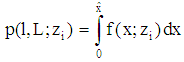is the probability of insolvency of the loan contract for the project ), (ii) The curves of the types are strictly monotonic increasing and strictly convex on . The mapping for all (the type i-line) is identical to the curve of a type i-firm at the level . (Note: is defined by ), and (iii) Since is a mps of the inequality is valid for all .

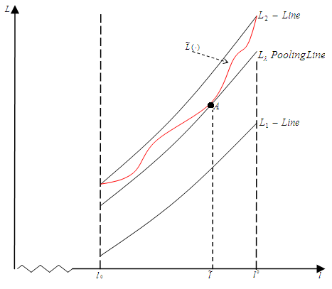Figure 2. No type-separation

Using the validity of in (iii) is proven indirectly. Two cases are to be considered. Case (a) If for all , then each PBE is of a pooling type. Suppose there exists a separating PBE with , , and . Due to (4), then we get 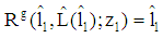and 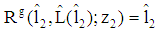. (Note: 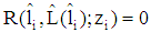holds according to 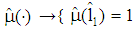, ). Thus, holds as well. Therefore, there is an incentive to deviate for a type 2-firm. (Note: If a type 2-firm asks for a loan with par value instead of , then a higher indifference curve is reached according to ).

We get a PBE of a pooling type with and if can be chosen such that the mapping on belonging to it is located beyond (see A in figure 2). Here, is given by and defines the so called “pooling line” for all . (Note: is given by for all ). Due to (4), satisfy . (Note: A choice is possible if the indifference curve of a type 1-firm at (see A in figure 2) does not intersect for all (type 2-line) since must be satisfied for all due to (4)).

This case occurs if the project with lower risk has lower probability of insolvency for all contracts with and must hold (see (6)). If , then is an equilibrium of a pooling type for all loans since the indifference curve of a type 1-firm does not intersect the indifference curve of a type-2 firm at . (Note: is defined by (the pooling condition) and 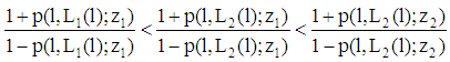for all holds since the slope of for all (type i-line) is given by . Hence, the slope of the indifference curve of a type 1-firm is always smaller than the slope of the indifference curve of a type 2-firm).

Remark 3 (i) In case (a) we discussed for all . If PBE exist, then they are of a pooling type. In equilibrium, the ratio chosen by the firm does not have the separation property. (Note: There are no schemes putting incentives for both types of the firm by which the self-selection property of the ratio leads to the disclosure of the firm’s types. However, it is obvious that signalling of the real type is in a type 1-firm’s interest (see figure 2)). (ii) PBE exist if for all loan contracts with and the less risky project has the lower probability of insolvency.

Finally, the extreme case (b) of a volume with is to be analyzed. Here, a separating equilibrium exists as well. Suppose there is any with . It is straightforward to see, if , , , and for all and if 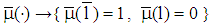for all and , then with is a PBE. According to (4), the system of beliefs and the strategy are consistent.

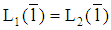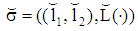Remark 4 (i) Each loan amount with generates a pooling PBE. (Note: By choosing and we get a pooling PBE with and 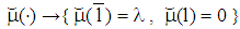for all with ). (ii) In case (b) a loan amount with 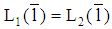is part of each pooling PBE. (Note: If a pooling PBE with , , , , and exists, then there is an incentive for a type 1-firm to deviate towards with (i.e., reaching a curve at level instead of a lower level is preferred by a type 1-firm). Note furthermore, is defined by and as well as must be satisfied necessarily). (iii) In all separating PBE a type i-firm gets the same expected payoff . This remains true for all pooling PBE. Thus, in case (b) all PBE are equivalent with respect to their payoffs. (iv) is valid for all loan amounts and claim schemes satisfying (4). The bank has no risk since the liable equity is sufficiently large. We have .

3. Concluding Remark

In a simple project funding game with limited liability and asymmetric information we deal with the question whether banks can conclude from the debt-to-equity ratio chosen by firms what projects’ risks will be. We cannot confirm a positive signalling result in general: all PBE are pooling equilibria if projects with continuously distributed cash flows are ranked according to second-order stochastic dominance and if the riskier project has a higher probability of insolvency for all chosen ratios larger than 1. This remains true if the less risky project has the higher probability of insolvency.

Appendix

Proposition 1 The slope of firm i’s indifference curve at is given by

Proof Let be the indifference curve of a type i-firm implicitly defined by if and let be denoted by . Then, the slope at is given by such that

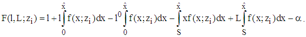Hence, according to 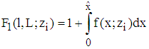and 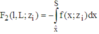we have

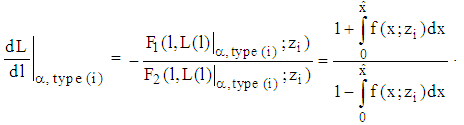Corollary The indifference curves of a type i-firm are strictly monotonic increasing

Proposition 2 The indifference curves of a type i-firm are strictly convex on

Proof Holds due to

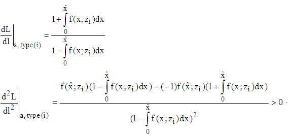Proposition 3 If is a mps of, then holds for all

Proof Suppose Proposition 3 does not hold, then 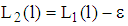must hold for any . Using 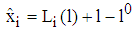and 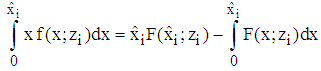we get

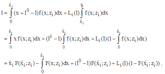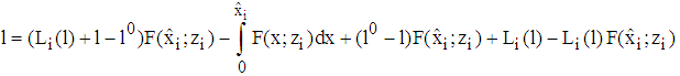
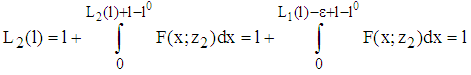
such that with , by conclusion, 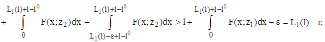holds as well. Here, the inequality is valid according to ssd. Hence, . This contradicts the assumption. Finally, it remains to be shown 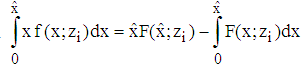. The anti-derivative of is given by 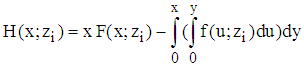according to

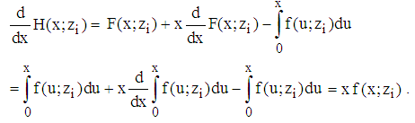Hence, .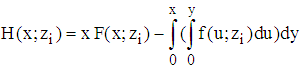