1. Historical Background

Games have been recorded throughout history but the systematic application of mathematics to games is a relatively recent phenomenon. Gambling games gave rise to studies of probability in the 16th and 17th century. What has become known as Combinatorial Game Theory was not ‘codified’ until 1976-1982 with the publications of “On Numbers and Games” by John H. Conway and “Winning Ways” by Elwyn R. Berlekamp, John H. Conway and Richard K. Guy. In the subject of “Impartial Games” (essentially the theory as known before 1976), the first MSc thesis appears to be in 1967 by Jack C. Kenyon and the first PhD by Yaacov Yesha in 1978 ([35]).

“Games of No Chance” are 2-player perfect-information games. A SUM of such games is naturally defined as the game in which each player at his turn may choose to make any of his legal moves on any single summand. The study of such sums is a subject called “combinatorial game theory“. The first part of Winning Ways [2nd edition, 2001-2004 provides a good introduction to this subject. Many research papers on this subject were presented at conferences held in 1994 and 2000 in Berkeley, CA, at the Mathematical Sciences Research Institute (MSRI) and at the Banf Research Center in Canada in 2005 and 2008 ([35]). Cambridge University Press later published proceedings of those conferences under the title “Games of No Chance (GONC)”. Aaron Siegel's “Combinatorial Game Theory” became the most definitive work on the subject when it appeared in 2013 ([35]).

The solution of the game of “NIM” in 1902, by Bouton at Harvard, is now viewed as the birth of combinatorial game theory. In the 1930s, Sprague and Grundy extended this theory to cover all impartial games. In the 1970s, the theory was extended to a large collection of games called “Partisan Games”, which includes the ancient Hawaiian game called “Konane”, many variations of “Hacken-Bush”, “Cut-Cakes”, “Ski-Jumps”, “Domineering”, “Toads-and-Frogs”, etc.… It was remarked that although there were over a hundred such games in “Winning Ways” ([35]), most of them had been invented by the authors. John Conway axiomatized this important branch of the subject. His axioms included two restrictive assumptions:

1. The game tree is LOOPFREE, so draws by repetitious play are impossible.

2. The NORMAL TERMINATION RULE states that the game ends when one player is unable to move, and his opponent then wins.

Games such as, “Checkers” satisfies the normal termination rule, but it is loopy. For example, if each player has only one king remaining, and each gets into a double corner, then neither player can bring the game to a victorious termination. “Dots-and-Boxes” on the other hand is loop-free, but it violates the normal termination rule because victory is attained by acquiring the higher score rather than by getting the last move. “Go” also fails to satisfy the normal termination rule, because the game ends when both players choose to pass, and then the winner is determined by counting score.

Most games on one side are fruitful targets for paper-and-pencil mathematical analysis, based on an ever-growing base of general theorems, but it seems the deeper you research the more you find that most games resist this approach, even in their late-stages. However, some of these games have succumbed to sophisticated computer attacks, which construct large databases of relevant positions.

Although chess definitely lies on the less theoretically tractable side, Noam Elkies composed some very clever “mathematical chess” problems, which fit the abstract theory of “Partisan Games”. He has also won the annual award of the international chess federation for the best chess problem composition. However, most chess masters see problems of this genre as only very peripherally related to real chess endgames ([35]).

When “Mathematical Go” began in 1989, it initially received a somewhat similarly skeptical reaction from professional Go players. However, as the mathematics expanded and improved, some scholars are now approaching the ability to analyze some real professional games and provide analyses, which are deeper and more accurate than those, obtained by human experts. The reason for this optimism is that virtually all “Go” endgames pass through a stage in which the play naturally divides into disjoint battlefields. A typical late-stage “Go” endgame on a single small battlefield is of at most modest complexity. In the early 1990s, new operators were introduced which map many such positions into the simpler games of “Winning Ways”. These mappings preserve winning strategies, and formed the original core of “Mathematical Go”, a subject which has continued to progress at a substantial rate.

The theory of “Mathematical Go” has advanced to the point that there now appear to be very promising prospects for combining it with some of the best tree-searching algorithms developed in the AI community. An initial goal would be a set of software tools which can analyze most championship-level “Go” endgames more accurately than any human. This could also have a big intellectual impact throughout East Asia, where the conventional wisdom still holds to the premise that “Go” demonstrates the superiority of “holistic” Asian thinking over the more “reductionist” approaches favored in the west.

There are two other branches of game theory, which have significantly different emphases than combinatorial game theory. One is called “Artificial Intelligence”, or AI. The AI approach to game-playing emphasizes very hard problems, including the play of openings and middle games which are so complicated that even the best human experts remain unsure whether any winning move exists or not. Limited search followed by heuristic evaluation and backtracking are the favored AI methods.

Many devotees of artificial intelligence hope or believe that there will be considerable commonality in the best programs for chess, checkers, Go, Othello, etc. (Since the chess victory of Big Blue over Kasparov, some of AI community's interest has shifted to “Go”, a game in which, as of 2016, thousands of humans can consistently beat the world's best current computer program). Skeptics see little such commonality in the best programs today. However, many adherents of both schools of thought share a common interest in tree-searching and tree-pruning algorithms, and in the potential to combine such algorithms with the decomposition algorithms of combinatorial game theory to provide the tools which will support computer attacks on much harder problems.

For the past couple decades, computer-based solutions to specific games on specific sizes of boards have been appearing faster than humans are digesting them. One of the first such was Oren Patashnik's solution of 4 x 4 x 4 tic-tac-toe. In the 1970s, he wrote a sophisticated program with which he interacted extensively for six months, and built up a large database of positions, which eventually became sufficient to prove that the first player could win. However, no human has yet learned to play this game perfectly without reference to the database ([35]).

The classical probabilistic theory of two-person games with chance and/or imperfect information is a third branch of game theory. This is the sort of classical von Neumann game theory in which several people, including John Hicks, Kenneth Arrow, John Harsanyi, John Nash and Reinhard Selten have won Nobel prizes in economics. This subject differs even more from combinatorial game theory and AI than the latter two differ from each other. Even so, there are some significant overlaps. Linear programming lies near the core of the classical probabilistic game theory. Linear programming also plays a much smaller but still significant role in combinatorial game theory (e.g., in one proof of one of D. Wolfe's theorems).

Most of the initial theoretical results of combinatorial game theory were achieved by exploiting the power of recursions. Combinatorial game theory has that in common with many other mathematical topics, including fractals and chaos. Combinatorial game theory also has obvious and more detailed overlaps with many other branches of mathematics and computer science, including topics such as algorithms, complexity theory, finite automata, logic, surreal analysis, number theory, and probability ([35]).

2. What is Combinatorial Game Theory?

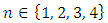
This Combinatorial Game Theory has several important features that sets it apart. Primarily, these are games of pure strategy with no random elements. Specifically:

1. There are Two Players who Alternate Moves;

2. There are No Chance Devices—hence no dice or shuffling of cards;

3. There is Perfect Information—all possible moves are known to both players and, if needed, the whole history of the game as well;

4. Play Ends, Regardless—even if the players do not alternate moves, the game must reach a conclusion;

5. The Last Move determines the winner—Normal play: last player to move wins; Mis`ere play last player to move loses!

The players are usually called Left and Right and the genders are easy to remember —Left for Louise Guy and Right for Richard Guy who is an important ‘player’ in the development of the subject ([39]). t. More on him is discussed later.

Examples of games1NOT covered by these rules are: DOTS-&-BOXES and GO, since these are scoring games, the last person to move is not guaranteed to have either the highest or the lowest score; CHESS, since the game can end in a draw; BACKGAMMON, since there is a chance element (dice); BRIDGE, the only aspect that this game satisfies is that it ends ([9]).

Games which are covered by the conditions are: NIM2; AMAZONS, CLOBBER, DOMINEERING and HEX. In fact, NIM, AMAZONS, DOMINEERING and also, despite the comments of the previous paragraph, DOTS-&-BOXES and GO have a property that makes the theory extraordinarily useful for the analysis of these games. The board breaks up into separate components, a player has to choose a component in which to play. Moreover, his opponent does not have to reply in the same component. This is why condition (4) is important. The aspect is so important that it has its own name. The disjunctive sum of games G and H, written G+ H, is the game where a player must choose to play in exactly one of G and H. The game of NIM with heaps of sizes 3, 4 and 5 is the disjunctive sum of three one-heap games of NIM. One could also imagine playing the disjunctive sum of a game of CHESS with a game of CHECKERS and a game of GO. On a move, a player moves in only one of the games but the opponent does not have to reply in the same game. The winner will be the player making the last move over all. As a rule-of-thumb, if a position breaks up into components so that the resulting game is a disjunctive sum then this theory will be useful. If the game does not become a disjunctive sum, HEX for example, then the theory is less useful. We still need a few more definitions. In an Impartial game both players have exactly the same moves—NIM for example. In a Partizan game the players have different moves—in CHESS a player can only move his own pieces and not those of his opponent; she would get rather upset if he did. A game belongs to one of four outcome classes. This was first noted, by Ernst Zermelo in 1912, but phrased differently ([14]). A game can be won by:

• Left regardless of moving first or second.

• Right regardless of moving first or second.

• By the Next player regardless of whether this is Left or Right.

• Or by the Previous player regardless of whether this is Left or Right.

Its initial usually refers to an outcome class. In an Impartial game such as NIM, since both players have the same moves thus the outcome of a position must be either N or P. A main aim of the theory is to give a value to each component: essentially how much of an advantage the position is to one of the players—positive value for Left and negative for Right. First, though, we have to deal with equality:

Two games should be the same if both players are indifferent to playing in one or the other. Or Equality or the ‘Axiom of In distinguishability’: G = H if, for all games X, the outcome for G + X is the same as the outcome for H + X.

Finally, we are ready to talk history! The history breaks up into three main threads and all threads are still very active:

• Impartial games under the Normal play ending condition which starts with Bouton and NIM through Guy & Smith

• Partizan games again under the Normal play rule starting with Milnor’s and Hanner’s work (from GO) through Berlekamp, Conway & Guy.

• Impartial games under the Mis`ere rules starting with Dawson in 1935. (See the Dover collection) What about the obvious fourth thread?

• Partizan Mis`ere games: there are exactly two papers on the subject, both in 2007. This topic is hard! Mathematical Interlude 1. How to play and win at NIM.

If there is one heap, take it all! If there are two unequal heaps, remove from the larger to leave two the same size. For three or more heaps, write each heap size as a sum of powers of 2, i.e., as sums of 1, 2, 4, 8, etc. pair off equal powers of 2; if all powers are paired off, invite your opponent to go first. He must disturb the pairings and your winning response is to remove enough counters to re-establish a pairing. Mathematically, write the numbers in binary and add without carrying ([9]).

For example: with heaps of size 1, 5 and 7 then as sums of powers of 2, 1 = 1, 5 = 4 + 1 and 7 = 4 +2 + 1, the 4s pair off but not the 2s or the 1s. The winning move (there could be more than one but not in this situation) is to play to remove 3 (=2+1) from the 7 heap to leave the position 1, 5, 4 where 1 = 1, 5 = 4 + 1 and 4 = 4. If the opponent were now to move to 1, 3, 4 then 1 = 1, 3 = 2 + 1 and 4 = 4 and only the 1s are paired. No move will ever create another 4 so the 4 has to go but at the same time you should leave a 2 to pair off with the other 2, i.e. move to the position 1 = 1, 3 = 2 + 1 and 2 = 2.

Figure 1. A diabolical disjunctive sum

3. Models of Combinatorial Games

Now we will show most of the combinatorial games, which previously studied, and we will try to explain the games in a brief ways.

3.1. Nim

Nim is a game where players take turns removing objects from different heaps (think stacks of coins). On a players turn, the player must remove at least 1 object from one of the heaps. They can remove as many objects as they want as long as they are in the same heap. The first player to be unable to move loses ([14]).

3.2. Toads and Frogs

Toads and Frogs is a game played on a 1×n strip of squares. Every square is either empty or has a toad or a frog. Players take turns, Left moving toads to the right if the next square is an empty square and right moving frogs to the left if the next square is empty. Also, if there is a frog in the square that a toad wants to move into, it can hop over the frog into the next square (2) squares ahead of where it started) if that square is empty. Similarly, a frog can jump over a toad to the next square if that square is empty. The first player that does not have a move loses ([14]).

3.3. Cut Cake

Cut Cake is a game played on a rectangular grid. During each players turn, they cut the rectangle into two smaller rectangles. The Left player can cut along the vertical (North to South) lines while Right can cut along the horizontal (East to West) lines. The first player without a move loses ([10]).

3.4. Hackenbush

Hackenbush is a game played on a configuration of colored lines (usually red, blue, and green). These lines are connected to the ground, either directly by touching the ground or indirectly by being connected to another line that is connected to the ground. Players take turns cutting the line segments ([3, 8, 28]) (i.e. erasing). The player Right can cut Red lines, the player Left can cut blue lines, and both can cut green lines. When a line is cut, any remaining pieces that are no longer connected to the ground are also removed. The first player to be unable to move loses.

3.5. Run Over

Run over is a game played on a finite strip of squares, where each square is empty or occupied by a Left or Right piece. Each player can move their piece one square to the left and replace any piece that is on that square. Once pieces reach the last square, they can move off of the board ([7]).

3.6. Date Game

This two players game starts with a date in January. Players take turns increasing either the month or the number, but not both. At any time, the applet is required to show a valid date. The player to reach December 31 wins the game. (To modify the date click repeatedly on either the month or the date and then press Move) ([7]).

3.7. Dawson's Chess

Dawson's Chess was invented in 1930s and is played with one or more heaps of items. The nature of the items is not important, but as in the game of Kayles they are referred to as Skittles. In the applet below, they are positioned on a circle, with the number of positions shown in the upper right portion of the applet. This may be specified by clicking a little off the vertical axis of the number. (Clicking to the left of the axis decreases the number, to the right increases it.)

To remove a skittle, just click on it. However, the rules devised by T. R. Dawson stipulate that, the immediate neighbors - if any - of a skittle that was clicked on are also removed. So that, depending on the configuration, a player may remove 1, 2, or 3 skittles ([45]).

3.8. Dawson's Kayles

Dawson's Kayles was invented in 1930s and is played with one or more heaps of items. The nature of the items is not important, but as in the game of Kayles they are referred to as Skittles. In the applet below, the skittles are positioned on a circle, with the number of positions shown in the upper right portion of the applet. Clicking a little off its vertical axis may specify this number. (Clicking to the left of the axis decreases the number, to the right increases it).

In Dawson's Kayles a player always removes exactly two adjacent skittles. Thus a lone skittle is a "dead weight" with the Grundy number of 0. The presence of a lone skittle, with no neighbors, does not affect the course of the game. To remove a pair of adjacent skittles, click somewhere between the two ([29]).

3.9. The Fraction Game

You are given several fractions that can be modified according to certain rules:

1. The number replacing a given one must have strictly smaller denominator, or,

2. If the denominator is already 1, it must have numerator strictly smaller in absolute value

There are two players: Left and Right. A replacement is only legal for Left if it decreases the number, legal for Right only if it increases the number. You choose to be either Right or Left and may force your computer to go first by pressing you move button. All numbers in the game are modified by clicking a little off their center line. Clicking on the right increases the number, clicking on the left decreases it. To perform a move, select a fraction, adjust it to the desired value and press the I move button.

The game has two parameters. Numbers is the number of fractions in a game. Max is the absolute maximum number that may appear in the numerator or denominator of a game. ([11])

3.10. Grundy's Game

Grundy's Game is played with one or more heaps of items. The nature of the items is not important, but in the applet below they may perhaps remind of chocolate squares. The only legal move in the game is to split a single heap into smaller two of different sizes. To perform a move click between any two (with the above provision) adjacent squares ([13]).

3.11. The Game of Hex

The game of Hex has been invented in 1942 by Piet Hein, reinvented in 1948 by John Nash, got its name in 1952 from a commercial distribution by Parker Brothers and has been popularized by Martin Gardner in 1957. In Hex, the player to make the first move has a better chance of winning than the other player. This follows by the strategy stealing argument invented by John Nash. Hence the first player has an advantage in the game. To compensate for this advantage in the applet below, the central cell is blocked for the very first move. Unlike chess or checkers, Hex can't end in a draw. You'll have to do your best to win against the computer ([17]).

3.12. Kayles

Kayles was introduced by Dudeney and Loyd. Two players take turns knocking down skittles - pins here in the US. Usually skittles are arranged in a row. In the applet below they make a circular pattern. With one ball a player may knock either 1 (a direct hit) or 2 adjacent skittles (hitting just in-between the two.) The players are so good at playing the game they can knock down the desired skittles at will. The last player to move wins.

(Clicking a little left or right off its centerline modifies the number of skittles. You can force the computer to make first move by clicking the start button) ([7]).

3.13. Nimble

The game of Nimble is much the same as the game of Scoring as we shall see later. The only difference is that now there is no limitation on the length of a move ([5, 14]).

3.14. Northcott's game

In every row of a rectangular board, there are two checkers: one white and one black. A move consists in sliding a single checker in its original row without jumping over another checker. You play white while the computer plays black. As usual, the player to make the last move wins ([17]).

3.15. Odd Scoring

The applet below serves a play board for a problem (Kvant, n 2, 1970, M8, p. 47) that I paraphrase the following way:

A chip is placed at the end of a grid band with N cells. On a move the chip is shifted leftwards 1, 2, or 3 steps. When it reaches the last cell, the total numbers of steps made by you and the computer are counted and the player who made an even number of steps is declared a winner.

The game is played against the computer. You move first.

To avoid a draw, the number of available steps is always odd. The idea is of course to devise a winning strategy ([16, 27]).

3.16. One Pile

One Pile is the most direct generalization of Scoring and the simplest of the Subtraction games. On each move a player is permitted to remove any number of objects bounded both from above and below. In the applet, a move is performed by pressing one of the buttons located on the perimeter of the drawing area. Clicking a little off their central line can modify the Min and Max attributes ([32, 33]).

3.17. Plainim

Plainim is played on a checkered board by removing or adding chips. There are just a few rules.

1. On a single move, one may only add/remove chips in a single row.

2. At most one chip is allowed per square.

3. One may only add chips to the right of a chip being removed on the same move.

4. The one to remove the last chip wins.

To perform a move click on squares (in a single row) where you want chips placed or removed (see that you confirm to Rules 1-3). Then press the button "Make Move" ([11]).

3.18. Plainim Misère

Plainim Misère is played on a checkered board by removing or adding chips. There are just a few rules.

1. On a single move, one may only add/remove chips in a single row.

2. At most one chip is allowed per square.

3. One may only add chips to the right of a chip being removed on the same move.

4. The one to remove the last chip loses.

To perform a move click on squares (in a single row) where you want chips placed or removed (see that you confirm to Rules 1-3). Then press the button "Make Move" ([15, 33]).

3.19. Scoring

The game of Scoring is very simple: the board is a strip of several squares (parameter Heap size), on which there are placed several chips (whose number is controlled by the parameter Counters). Taking turns with your computer you drag chips (one at a time) leftward until all are collected in the leftmost square. The last fellow to make a move wins ([19, 34]).

3.20. Scoring Misère

Misère games are played by the same rules as the normal ones with one notable exception: while in the normal game the player unable to move loses, in the misère games, the player unable to move wins.

In the Scoring misère, like in Scoring, the players are presented with one or more piles (or heaps) of objects (chips, counters, pebbles.) A move consists in removing a number of objects from a single pile. In Scoring (normal or misère), a player, on a single move, is allowed to remove one or more objects up to a prescribed maximum.

Strangely, the misère games are by far more difficult than their normal counterparts. A winning strategy is known for the straight Nim and its various incarnations (Nimble, Plainim, Date Game, or, say, Silver Dollar Game with No Silver Dollar.) For Nim, the winning strategy is to play as in normal Nim until all non-empty heaps with one exception, contain a single counter. Then make a move so as to leave an odd number of single counter heaps.

Scoring, especially with several heaps, is often (and mistakenly) identified with Nim. In particular, it is very easy to give an example when the above Nim misère strategy does not work for the Scoring misère. I've no doubt you would run into such a situation if you play with the applet below. (In addition to the above, it implements one other strategy and makes a random selection between the two) ([12, 28, 41]).

3.21. Scoring Misère: Two Heaps Perfect Strategy

Misère games are played by the same rules as the normal ones with one notable exception: while in the normal game the player unable to move loses, in the misère games, the player unable to move wins.

In the Scoring misère, like in Scoring, the players are presented with one or more piles (or heaps) of objects (chips, counters, pebbles.) A move consists in removing a number of objects from a single pile. In Scoring (normal or misère), a player, on a single move, is allowed to remove one or more objects up to a prescribed maximum. In the misère game, the player who was forced to remove the last item loses.

Unlike the normal games, the misère does not in general have a perfect strategy. However, in case of just two heaps a perfect strategy does exist.

The MAA Math Horizons magazine (v 17, n 4, April 2010, pp. 31-33) posted a solution to the problem by Dan Kalman and Michael Keynes of American University Which is called Double Take:

Starting with two non-empty stacks of chips, one of size m and the other of size n, the two players alternate turns and take 1, 2, or 3 chips from a single stack on each turn. The loser is the player who removes the last chip out of the initial m + n chips. Find the values of m and n that guarantee that the second player wins with best play.

In the problem, the players are allowed to remove maximum of 3 chips. In the applet this restriction is removed and you can specify the maximum move of any size - in principle, of course. For technical reasons the applet allows removing at most 10 chips. The chips are represented by small squares lined in a row (a heap). The squares are counted left to right. To remove a desired (but legal) number of squares click on the first one to be removed ([12, 28, 21]).

3.22. The Silver Dollar Game

This game adds a twist to the bogus Nim. One of the counters - a Silver Dollar - is different. A counter may be only moved leftward without jumping over other counters. Also, as before, no two counters may occupy the same square. The leftmost square is the only exception to that rule. The leftmost square may contain any number of counters. The purpose of the game now is to gain possession of the Silver Dollar.

The cherished coin may only be removed from the leftmost square. The game has two variants. In the first, the player who places the Silver Dollar on the leftmost square earns the right to grab it on the same move. In the second variant, removal of the Dollar takes two steps. After one player is forced to place the Dollar on the leftmost square, the other player wins by picking it up on his turn ([31]).

3.23. The Silver Dollar Game with No Silver Dollar (Bogus Nim)

This game is played very much like the games of Nimble and Scoring. Counters are placed on strip of squares and are moved (dragged) leftward. Counters are not allowed to move over each other, and no two counters may be placed on the same square ([31, 36, 41]).

3.24. A Sticky Problem

The game presented by a Java applet below was published in 2002 the American Mathematical Monthly as problem 569 (Sung Soo Kim). A solution by Li Zhou appeared in v. 111, n. 4 (April, 2004), pp. 363-364.

A game starts with one stick of length 1 and four sticks of length 4. The two players move alternately. A move consists of breaking a stick of length at least two into two sticks of shorter lengths or removing n sticks of length n for some . The player who makes the last move wins. Which player can force a win, and how?

The applet allows one to start with different initial configurations, but also with the standard one. At the outset, you can force the computer to make the first move by pressing the "Make move" button. Sticks are represented by a row of small squares that might remind of a chocolate brick. To break a piece click on a square to the right of the desired break line ([23, 37]).

3.25. Another Sticky Problem

The game presented by a Java applet below was published in 2004 the Mathematics Magazine as problem 1687 (Sung Soo Kim). A solution by Li Zhou appeared in v. 78, n. 1 (February, 2005), p. 70.

A two-player game starts with two sticks, one of length N and one of length N+1, where n is a positive integer. Players alternate turn. A turn consists of breaking a stick into two sticks of positive integer lengths, or removing k sticks of length k for some positive integer k. The player who makes the last move wins. Which player can force a win, and how?

The applet allows for experimentation with different starting lengths. At the outset, you can force the computer to make the first move by pressing the "Make move" button. Sticks are represented by a row of small squares that might remind of a chocolate brick. To break a piece click on a square to the right of the desired break line ([22]).

3.26. Subtraction Game

In the Subtraction Game you are given a number of minuends and a number of subtrahends. Players take turns subtracting subtrahends from minuends - one subtraction at a time. Only non-negative results are legal. The player unable to move loses. A horizontal line separates minuends (placed above the line in a rectangular array) from subtrahends (always located in a row below the line).

To perform a move, select a minuend and then click on a subtrahends.

The game has three parameters. Nums is the number (from 1 through 12) of minuends to subtract from. Subs is the number (from 1 through 8) of possible subtrahends to be subtracted from minuends. Max is the absolute maximum of minuends. Subtrahends may change between 1 and 9 (inclusive). They may be modified when the Define button is checked.

The numbers that could be modified (Nums, Subs, Max and subtrahends) by clicking a little off their vertical central line. Clicking on the right from the line increases the number, clicking on the left decreases it.

When subtrahends form a sequence of consecutive numbers starting with one, the game is equivalent to Scoring. Since the players are free to define subtrahends to their liking, Subtraction Game is more general ([24, 41]).

3.27. TacTix

TacTix is a derivation from Nim invented by Piet Hien in the late 1940s. It is played on a N×N board filled with chips. At a turn, a player removes a number of contiguous chips from a single row or column. TacTix's normal game is trivial: if N is odd there is a winning strategy for the first player; if N is even there is a winning strategy for the second player. (In both cases, the clever player would utilize the central symmetry of the board.) Hence, TacTix is played in itsmisère variance: the player to pick the last piece loses the game ([25]).

3.28. Take-Away Games

Like One Pile, the Take-Away games are played on a single pile of objects. On the first move a player is allowed to remove any number of objects, but the whole pile. On any subsequent move, a player is allowed to remove any number of objects bounded from above by a quantity that depends on the previous move.

The applet below implements three such games. In one, a player can remove no more than what his or her opponent removed on the previous move. In the second game, the condition changes to less than twice of the previous move. An in the third, it's no more than twice the previous move ([24, 44]).

3.29. Turning Turtles

At each move a player chooses an "O" and turns it into an "X". At the same time this player may, if he so wishes, changes a letter in any other square to the left from the first one. In the left square, the player is allowed to turn "O" into "X" and also "X" into "O". To perform a move, the player should first click under the square he plans to change. After selecting 1 or 2 squares, click on the "Make Move" button. If you plan to change a single square (an "O" into an "X") you may click on that square directly. This is kind of a shortcut with which one should be cautious. You can't undo your moves. The player to make the last move wins.

In the original version, players turn turtles upside down and back to their feet. Not having any aptitude for painting, I settled on the Tic Tac Toe symbols to present the two possible states of each square ([26]).

3.30. Wythoff's Nim

The game below has no traditional name, was invented at about 1960 by Rufus P. Isaacs, a mathematician at Johns Hopkins University. It is described briefly in Chapter 6 of the 1962 English translation of The Theory of Graphs and Its Applications, a book in French by Claude Berge. Let's call the game "Corner the Lady." Computer puts the queen on any cell in the top row or in the column farthest to the right of the board; Queen's location is designated by the red square. The queen moves in the usual way but only west, south or southwest. Eligible squares are colored in magenta. You click on one of these to select a move. You move first, and then the computer and you alternate moves. The player who gets the queen to the lower left corner is the winner. No draw is possible, so that one of the players is sure to win ([15]).

3.31. Wythoff's Nim II

This is a second and a more direct implementation of Wythoff's Nim. To remind, the players take turns removing any number of objects from one of the heaps, or removing the same number of objects from the two heaps simultaneously.

In the applet objects are removed from the right. Click on the last square you want removed. If the box "Two heaps" is checked, the same number of objects will be removed from both heaps regardless of which one you click upon ([15]).

4. Comparison of Some Games

From a mathematical point of view, we note that combinatorial games can be classified into several categories.

The first category can be dealt with algebraically, where we can analyze and find appropriate algorithms to solve the game. For example, “Nim” is a game, which has a clear connection with the mathematical binary system. You can clearly find the correct winning strategies by understanding the mathematical binary system.

The second category can be dealt with graphical or engineering methods. For example, “Hackenbush” is a game, where graphical knowledge can explain the winning solutions, step by step.

The third category is more complicated, such as “Chess”, which requires knowledge in different mathematical concepts and methods to develop correct strategies to win the game.

5. Game Rules and Game abbreviations

We will try to explain how to deal with the Games and we'll show the rules.

5.1. Various Game Values

If we have a game G and this game and This game include options for player L named and options for player R named :

Equivalently, if has the same outcome in best play as for all games K

If , then the first player to move loses

A positive game value is a Left win

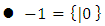A negative game value is a Right win

From the above, we find:

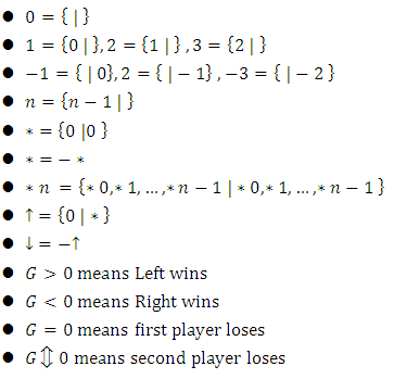In another way

l Zero: If G is a 2nd player wins then the outcome of is the same as that of H for all games H. The player who can win H plays this strategy and never plays in G except to respond to his opponent’s moves in G. Thus, any 2nd player wins game acts like 0 in that it changes nothing when added to another game.

l Negative: Given a game G, - G is G with the roles reversed. For example, in CHESS this is the same as turning the board around.

l Equality: if is a 2nd player win; i.e. neither player has an advantage when playing first. Note this is a ‘definition’ of equality and mathematically we can say is the same as . (Note that: this really defines an equivalence relation and the ‘equality’ is for the equivalence classes).

l Associativity is straightforward from the definition of the disjunctive sum; 5. Commutativity:, again straightforward;

l Inverses: For any game is a 2nd player win, by ‘Tweedledum-Tweedledee’. Whatever you play in one, I play exactly the same in the other.

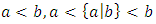
l Inequality: if the Left wins ; i.e. there is a bigger advantage to Left in G than in H.

The structure really is a partial order. For example, when playing NIM, a heap of size 1 and a heap of size 2 are incomparable. Let’s call these games and for easy reference. Note that is the same game as since the Left moves are the same as the moves available to Right so interchanging them has no effect on the play of the game. We already know that a first player win, the winning move is to . According to the definition of ‘equality’ then . 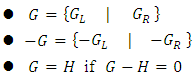Moreover, according to the definition of inequality and ([26]).

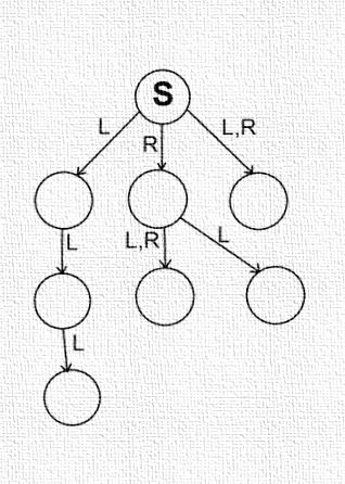Figure 2. Sample Game with Two players, left and right, alternate moves

If you have no move, you lose and your opponent wins and games must terminate in finite time.

5.1.1. Definition

A game is an ordered pain of sets of games and we write a game as { left's moves | right's moves } Or { left's options | right's options } Or 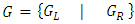([5.6]). For example the empty set of games, so is a game, won by the second player. We now have two sets of games: and , so we can form games left wins right wins first player wins We now have 16 set of and we can write:

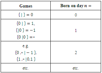
5.2. Addition

In the sum of two games , a player may move in either x or y, leaving the other unchanged, more formally ([7]).

Definition

Note: Game is born on the sum of the days on which x and y are born.

5.2.1. Properties of Addition

5.2.1.1. Theorem Addition is Commutative.

Proof Base case: 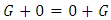for all games G.

Induct on the sum of days on which x and y are born:

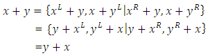5.2.1.2. Theorem Addition is associative ([9])

5.3. The Negative of a Game

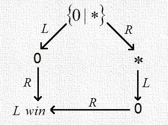
5.3.1. Definition

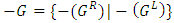The effect is that all moves of Left and Right are switched ([26]).

is a second player win. For example in Fig. 3, Right first:

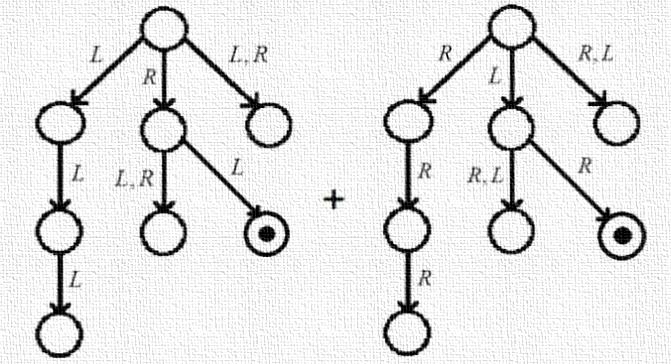Figure 3

Right to move, so Left wins.

5.4. Zero Games

Note that is not the same as 0!

5.4.1. Definition

l A game is a zero game if it is a second player win.

l Define to mean that is a zero game ([40, 48]).

5.5. Comparing Games

5.5.1. Definition If is positive then .

For example is a Left win, so .

and is fuzzy, so * and 0 are not comparable. So games form a po ''set'' ([9]).

5.5.2. The Game "2"

Let .

Analyze the game , see Fig .4 to find , so

Figure 4

5.6. Ordinals

5.6.1. Definition

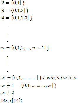for example Consider the game

see Fig .5 to find that it is positive:

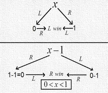Figure 5

5.6.2. What is

Figure 6

5.7. Making More Games

Let . As before, we can show .

In fact. 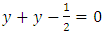, so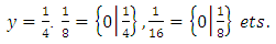

In this way we can construct games corresponding to

Recall that we have also constructed a game for every ordinal number. Now let’s combine all the games we have so far ([20, 38]).

5.8. Multiplication

For numbers or, if are surreal,

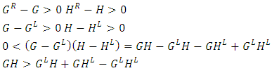Similarly

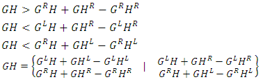5.8.1. Properties of Multiplication

Can prove the following by induction

l Well defined

l Distributive law

l Associative

l 1 is the multiplicative identity

l Commutative

l Every nonzero surreal has an inverse

So the surreal numbers are almost a field ([6, 17, 42])

5.9. Other Games

Consider the game . It is not a number because

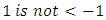We compare to a number x with in Fig .7.

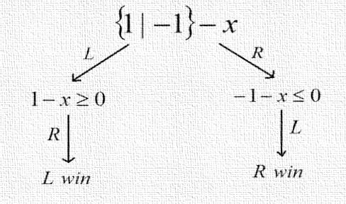Figure 7

So is fuzzy (a first player win). Because the first player move with .

Note that In a number x , nobody wants to move because and .

More on

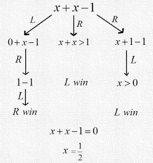
In Fig.4 we have shown that is not comparable to numbers . For , then

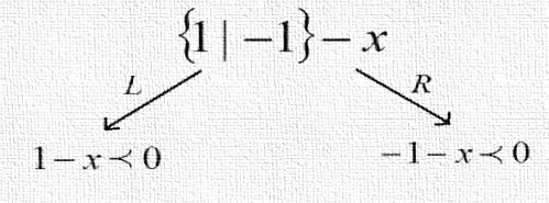Figure 8

Is a right win, so

In Fig .9 note that so also

Figure 9. Relating to surreals

Any game born on a finite day corresponds to a cloud with dyadic endpoints.

If two games overlap, they are not comparable, if they do not overlap, you can compare them ([1, 2]).

5.9.1. Lemma

For any game G, there is an ordinal such that

Proof

If G is born on day n, choose . Game G will turn to 0 in at most n moves.

Left wins by always moving in . He will always have a response to a move in G. So

. In Fig .10 note that similarly .

Any game corresponds to same cloud.

If two games overlap, they are not comparable. If they do not overlap, you can compare them ([42, 43])

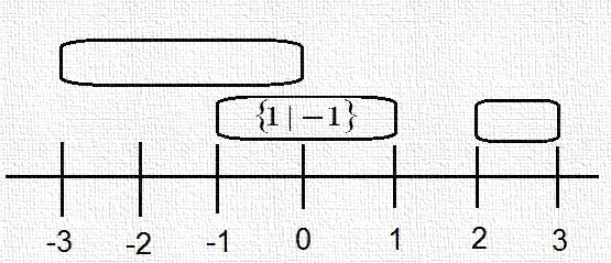Figure 10

5.9.1.1. Where is *?

Recall that is fuzzy with 0.

5.9.2. Lemma

If is a number, then is a left win.

We will Proof that in Fig .11

Figure 11

Since x is a number,

* is not comparable to 0.

For a number , since positive we get .

Similarly, * is greater than all negative numbers. So * forms a cloud all at 0 , see Fig .12 to find it ([4]).

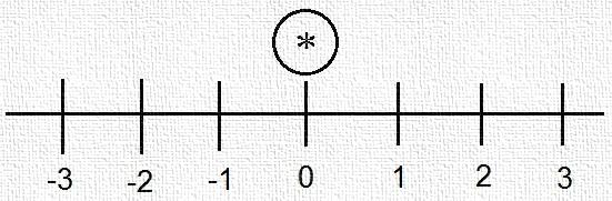Figure 12

Impartial games, means game G is impartial if and are identical and impartial. We write , where are the options of G.

is a zero game:

5.9.3. Definition

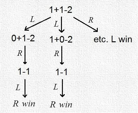
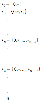each of these has a cloud all at 0 ([46]).

5.9.4. All stars are different

If n >m then see Fig .13 to find that is a first player win.

Figure 13

So far two different ordinals n and since the difference is fuzzy ([30, 47]).

5.9.5. Terminology

These games are also called Nim piles

Another small game:

Figure 14. Nim piles

So ([22. 34]).

6. Some Applications

After we learned about the combinatorial games and how to deal with the games in algebraic ways, We will talk about some of the chess-related applications, which is one of the most important applications.

6.1. The Chessboard Problems

For more than 250 years, combinatorial problems on chessboards have been studied and published in numerous books on recreational mathematics. Two problems of this type include the problem of finding a placement of n non-attacking queens on an chessboard and the problem of determining the minimum number of queens who are necessary to cover every square of an chessboard. Within the past five years a surge of interest in chessboard problems has occurred among a group of a dozen or so graph theorists and computer scientists. This paper surveys recent developments and mentions a large number of open problems. Combinatorial lists and puzzle-solvers have studied combinatorial problems on chessboards for over 250 years. Investigations center on the placement of the various types of chess pieces, viz, kings, queens, bishops, rooks, knights and pawns, on generalized chessboards ([47, 48]).

6.1.1. The Knight’s Tour

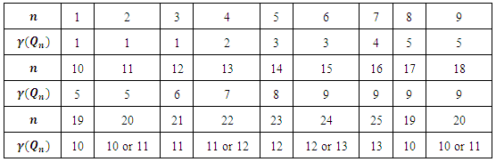
The closed knight's tour of a chessboard is a classic problem in mathematics. Can the knight use legal moves to visit every square on the board and return to its starting position? The unique movement of the knight makes its tour an intriguing problem, which is trivial for other chess pieces (Fig. 15). The knight's tour is an early example of the existence problem of Hamiltonian cycles. So early, in fact that it predates Kirkman's 1856 paper, which posed the general problem and Hamilton's Icosian Game of the late 1850s ([47, 48]). Euler presented solutions for the standard 8_8 board and the problem is easily generalized to rectangular boards. In 1991 Schwenk completely answered the question: Which rectangular chessboards have a knight's tour? Schwenk's Theorem: An chessboard with has a closed knight's tour unless one or more of the following three conditions hold:

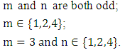The problem of the closed knight's tour has been further generalized to many three- dimensional surfaces: the torus, the cylinder, the pillow, the Mobius strip, the Klein bottle, the exterior of the cube, the interior levels of the cube, etc. Watkins provides excellent coverage of these variations of the knight's tour in Across the Board: The Mathematics of Chessboard Problems. However, the general analysis of these three- dimensional surfaces are to unfold them into the two-dimensional plane, apply Schwenk's Theorem as liberally as possible and tidy up any remaining cases as simply as possible. While this technique is successful at obtaining complete characterizations in some set- tings, it does not adequately tackle every surface and leaves the reader wondering what could be accomplished with a true three-dimensional technique ([47, 48]).

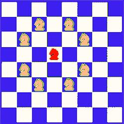Figure 15. Knight’s moves

6.1.2. The Domination Problem

The classical problems of covering chessboards with the minimum number of chess pieces (P) were important in motivating the revival of the study of dominating sets in graphs, which commenced in the early 1970’s. These problems certainly date back to de Jaenisch and have been mentioned in the literature frequently since that time.

The domination means that all vacant positions are under attack. This problem is called the domination number of problem and this number is denoted by . The number of different ways for placing pieces of P type to obtain the minimum domination number of P in each time denoted by . Also, the researchers are interested in the domination number of two different types of pieces by fixing a number of one type P of pieces and determine the domination number of another type of pieces. Finally, they compute the number of different ways to place the minimum number of pieces with a fixed number of pieces to dominate the chessboard.

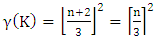
Theorem 6.1.2.1 The domination number of K pieces with fixed pieces of R in a square chessboard of size n is given by

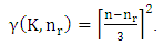(5.6)

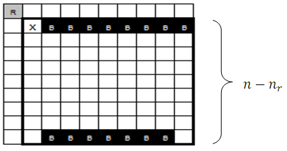
Proof: We know that by equation (1.5) in a square chessboard of size n. If we distribute the K pieces in the chessboard as minimum dominating distribution and place the R pieces in 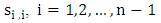in order to keep the minimum number of domination (any other placing make a partition on the chessboard). According to these placing of R pieces, then we get the maximum of for these pieces, and a square chessboard of length of cells which are not attacked.

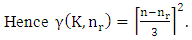There are several distributions for B pieces and all these distributions lead to the same conclusion, therefore we will take any one of them to complete the calculations. Therefore, in the following theorem, we will take any of the different cases of distribution of B pieces to find results.

Example: Given an board, find the domination number, which is the minimum number of queens (or other pieces) needed to attack or occupy every square.

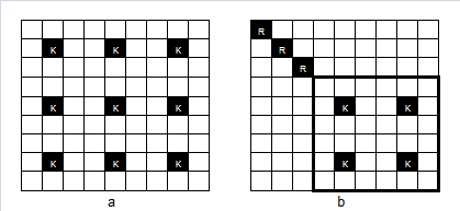Figure 16&17. (a) The minimum dominating K pieces in chessboard of size 9 (b) A distribution of K pieces with fixed number of R pieces

Figure 18. Domination of the Chessboard with 5 Queens

Table 1. Known Domination Numbers

Figure 19. Eight queens problem

6.1.3. The Eight Queens Problem

The eight queens puzzle is the problem of putting eight chess queens on an chessboard such that none of them is able to capture any other using the standard chess queen.s moves. The colour of the queens is meaningless in this puzzle, and any queen is assumed to be able to attack any other. Thus, a solution requires that no two queens share the same row, column, or diagonal.

The eight queens puzzle is an example of the more general n queens puzzle of placing n queens on an chessboard.

6.2. Independence of B Pieces with a Fixed Number of R Pieces

We denote the Independence number of B pieces with a fixed number of R pieces by .

Theorem 6.2.1. The independence of B pieces with a fixed number of R pieces is given by

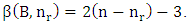(5.5)

Proof: The idea is to place pieces of R and then we distribute the B pieces to get the independence number of the B pieces together with a fixed number .

We place the R pieces in suitable cells that in the main diagonal of a square chessboard 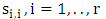in order. Since in this cell the R pieces take the maximum , and no make partition to the chessboard that contains from the cells which are not attacked by these pieces. This chessboard forms a square chessboard of length . We know that 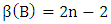by equation (1.4), where n is the size of the square chessboard. So we distribute 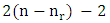in the chessboard of size , but we must remove the B piece from the main diagonal, since it is attacked by the R pieces. Thus we get:

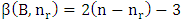The following example illustrates the application of the above theorem for different values of .

Example 6.2.2

For and , using the equation (5.5), it is obtained that ,

Figure 20. A distribution of B pieces with fixed pieces

7. Conclusions

In this paper, we have explained some models of combinatorial games, and we did perform a simple comparison between them. Then we have introduced the games’ rules and how to add, multiply and compare them. We have also noted how to implement what we have discussed into a mathematical environment, and finally gave some examples of those processes over some chess games such as, “The Knight’s Tour'','' The Domination Problem '', and'' The Eight queens Problem''.

8. Future Potential Topics

We noticed that there are a number of mathematical operations such as, addition and multiplication. We find for every game “G” there is – G where G – G = 0, which leads to a conclusion that can be discovered. Is there a group that can be defined as “Games” which consists of different games as elements, and does that group is an algebraic structure?.