Essam EL-Seidy1, Mohamed Mamdouh Zayet2, Hassan El-Hamouly2, E. M. Roshdy2
1Department of Mathematics, Faculty of Science, Ain Shams University, Cairo, Egypt
2Department of Mathematics, Military Technical College, Cairo, Egypt
Correspondence to: Essam EL-Seidy, Department of Mathematics, Faculty of Science, Ain Shams University, Cairo, Egypt.
| Email: |  |
Copyright © 2016 Scientific & Academic Publishing. All Rights Reserved.
This work is licensed under the Creative Commons Attribution International License (CC BY).
http://creativecommons.org/licenses/by/4.0/

Abstract
Game Theory is of interest because it is utilized extensively in many applications such as insurance, business, military and biology. One of the famous examples that has been investigated and analysed widely by game theory is the Iterated Prisoner Dilemma (IPD). Many researchers tend to change the IPD memory, due to the lack of information or the delay that may occur in cases that need a quick firm decision. Up till now there is no detailed investigation of using the outcome of the second-previous round (memory two) instead of the immediately-previous one. In this study, the critical role played by only a finite two state automata is presented due to the exponentially increase of number of strategies with number of rounds. One of the greatest challenges is the noise occurred during implementation. Therefore, this paper traces the development of strategies payoffs under noise using second-previous state. It will be argued that the payoff matrix will be analysed to illustrate strategies behaviour. The objective of this study is to investigate mixed strategies between all heteroclinic three-cycles. The results showed that neither strategy abide in front of all other strategies, however there are four strong strategies. A case study is adopted to examine the strategies behaviour in business cooperation conflict.
Keywords:
Iterated games, Prisoner's dilemma, Finite automata, Game dynamics, Transition matrix, Perturbed payoff
Cite this paper: Essam EL-Seidy, Mohamed Mamdouh Zayet, Hassan El-Hamouly, E. M. Roshdy, The Effect of Memory Change in Iterated Prisoner Dilemma Strategies Behaviour, Journal of Game Theory, Vol. 5 No. 1, 2016, pp. 1-8. doi: 10.5923/j.jgt.20160501.01.
1. Introduction
Complexity of computations and calculations of many mathematical models forces mathematicians to find a new technique. Game Theory is one of these new techniques that were implemented to beat these difficulties in conflict situations. The first serious discussions and analyses of cooperative games emerged during the 1950s by Von Neumann [1]. Also, Noncooperative games was reported in the first studies of Nash [2]. Then several studies follow the steps of Von Neumann and Nash. Insurance, business, military, and biology are some of the fields in which rational decision making is needed [3-10]. Game is a competition between players seeking objectives. Games can fall into main two types, game of chance such as roulettes or game of strategies such as poker. Game of strategies is the game of interest in this study. The main task is to get the strongest strategy that maximize the payoff and minimize the loss of each player. Prisoner Dilemma (PD) is a simple form of a two player-game and it could be considered one of the most frequently used example that arises in many applications [11, 12]. PD is a competition between two players (prisoners) each of them facing an indictment of a crime. Each player has one of two decisions to cooperate (deny) (C) or defect (confess) (D) with the other player. Both players are rewarded (R) if both of them cooperate. In turn they are punished (P) if both of them defect [5, 13]. In case of opposite decisions the co-operator is suckered (S) and the defector is tempted (T). PD has two main conditions T>R>P>S, and 2R>T+S. These conditions mean that the player who chooses mutual cooperation receives a payoff higher than switching between cooperation and defection [14]. The following payoff matrix is a good illustration of the PD game. | (1) |
To date, several studies used the immediate-previous state (memory one) to generates the new state. Many researchers tend to change the IPD memory, due to the lack of information or the delay that may occur in cases that need a quick firm decision. So a quite modification is used in this work, where the second-previous round (before the last one) was used to get the new state. Consequently sixteen sequences arise due to the imposition of the first two rounds. In this paper the third state is generated using the outcome of the first one and the fourth state using the outcome of the second one. This algorithm will be repeated infinitely then the average payoff is calculated using the payoff of each round. A notable example of two length memory is the conflict between two companies. If these companies have mutual three projects. The first project decision and payoff is known. Then however, the decision of the second project was taken it isn’t known for the other company. Finally there is new decision must be taken in the third project. So the new decision depends on the second-previous project outcome.The number of strategies that can be used is very large [10, 15-18]. A two-state automata is adopted to represent the strategies that were only used in this work. The total number of two state automata strategies is sixteen strategy [19]. Conflicts of every strategy with the other strategies are studied and payoffs are recorded in 16 × 16 matrix.Payoff matrix of 256 entries is constructed under the effect of noise (error in perception or implementation) [13, 19]. Optimum strategy which will invade all the other strategies is hoped to be determined. But unfortunately neither strategy abides in front of all other strategies. Further analysis shows that two or more strategies can be mixed with different probabilities to get better results.The equilibrium between a number of strategies more than three is time consuming and very complex. Only mixed strategies between heteroclinic three-cycles are calculated. If there are three strategies A, B and C where A invades B and B invades C and C return to invade A this is called heteroclinic three-cycles. Every equilibrium point between all heteroclinic three-cycles is calculated for Axelrod's values (T=5, R=3, P=1, S=0) [3, 20]. This will be carried out using game dynamics. Interestingly, some weak strategies in memory one do better in case of memory two.
2. Average Payoff
Iterated Prisoner Dilemma of memory two is represented as a first step to increase the memory of Prisoner Dilemma which arises in many applications. The approach of this paper depends on using the second-previous state outcome. Thus the third state is generated using the outcome of the first one and the fourth state using the second one. The unknown immediately-previous state outcome due to lack of knowledge or delay is the main reason to use the second-previous one. This algorithm will be repeated infinitely then the average payoff is calculated using the payoff of each round.There are an infinite number of strategies that can be used by each player. Studying these strategies will be very complex and time consuming. Only strategies generated by a two state automata will be studied to minimize calculations. Two state automata Figure 1 is a simple graph used to generate the new state from the known state. There are two nodes in each two state automata C and D exiting from each node two edges marked by C and D. There is an additional arrow to illustrate the imposition of the first state [13]. Two state automata generates only sixteen strategies that will be studied. 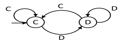 | Figure 1. Automata of TFT(1,0,1,0) strategy (S10 player imitating the adversary’s previous move) |
The couples 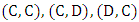 and
and  are the alternatives outcomes of each round. These couples consist of the decisions of the two players corresponding to the specified payoffs
  and
and  respectively. Binary system will be used to represent the sixteen strategies as quadruples of zeros and ones. Every digitrepresents the reaction of the player when one of the 4 possible outcomes of the known round arises
  . Zeros and ones indicate the player next move will be D for 0 and C for 1. The quadruple
  is called the Grim strategy and is the binary representation of
  and
and  is called Tweedledee and represents
  . The conflict between
  against
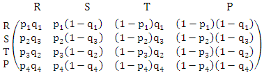
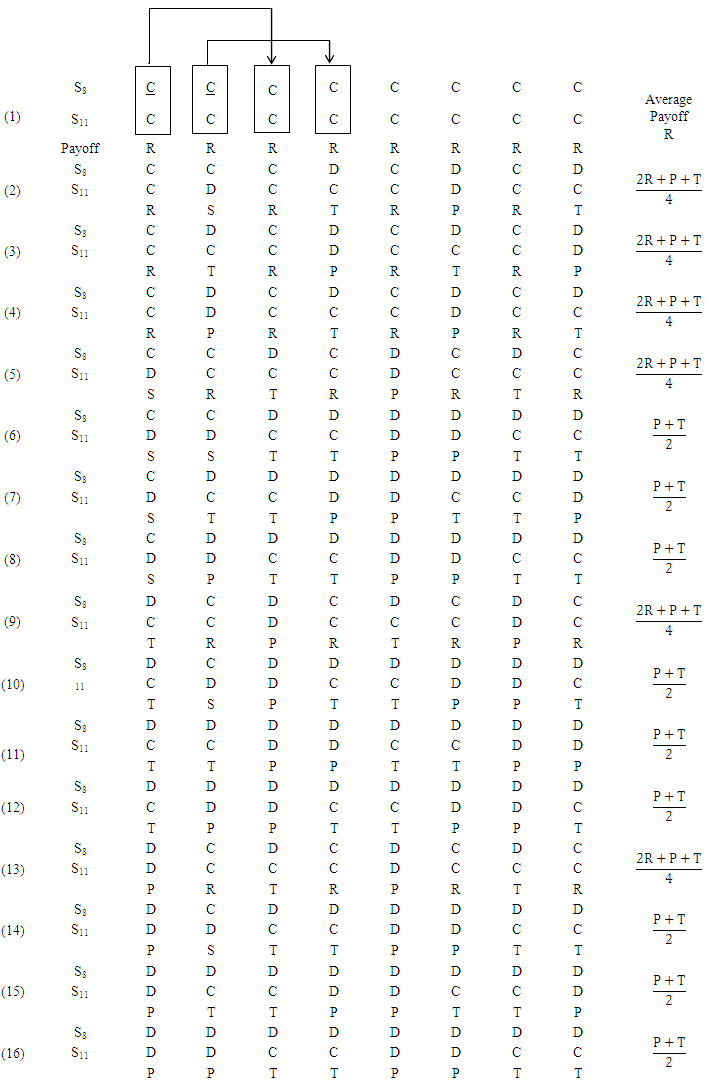
  is shown in Illustration 1.The Illustration 1 gives the alternative sequences by which the game may be started (exactly sixteen sequences). Every one of the sixteen sequences has one of three average payoffs for S8 player, R (Regime A) for sequence number 1 only,
 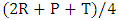 (Regime B) for the sequences 2, 3, 4, 5, 9, and 13, and
  (regime C) for the others.
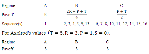 The three payoffs are equal, then starting with defection for S8 player (may be a company) is better than cooperation. So starting with defection for company using strategy S8 against S11 is the best choice to avoid cooperation risk. The recent important question is what the effect of noise in player (company) that plays with S8strategy?
3. Perturbed Payoff (Noise Effect)
Existing of errors (noise) due to implementation may affect the average payoff. To calculate the perturbed payoff, let there is a player playing by strategy 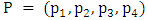 against another which playing by strategy
 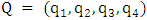 where Pi and Qi represents the probability to play C after every outcome
  respectively. Transition matrix can be constructed using the transitions between the available states
 | (2) |
 | (3) |
Since pi, qi are zeros or ones, then in some cases the stochastic matrix (2) will contain many zeros, and it is no longer irreducible. Therefore, the vector π is no longer uniquely defined.Now, we are going to use another direct technique to compute the stochastic vector II. Let us exemplify it for S8 against S11 as following. Every regime will be studied separately.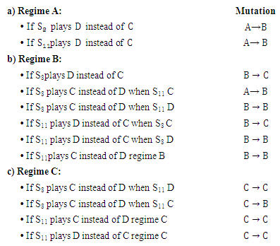 Thus the corresponding transition matrix from one regime to another will be as follows.
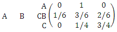 | (4) |
The triples  is the corresponding stationary distribution for perturbed S8 against S11. The perturbed payoff will be calculated by equation (5).
 | (5) |
The payoff of every entry of the 256 entries matrix will be calculated by the same method and recorded in Table 1.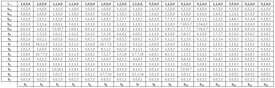 | Table 1. 16×16 Payoff Matrix |
4. Game Dynamics
Domination is the main invasive method to determine the strongest stable strategy. Does  dominate
  ? To answers this question firstly four payoff values of
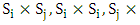
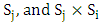 must be extracted from Table 1. Then these payoffs are used to form a new 2×2 matrix.
 | (6) |
Then if  and
and  , with at least one inequality being strict this means that
  dominates
  [13]. This algorithm will be repeated for each strategy in two cases:1. For the following conditions (suitable conditions):a) T > R > P > S.b) 2R > T + S.c) 2P < T + S.d) 2P > R + S.e) T + S < R + P.f) R + 3P > 2T + 2S.g) R – S > 2T – 2P.h) 4T – 4R > 3P – 3S.2. For Axelrod’s values (T = 5, R = 3, P = 1,S = 0).Table 3 illustrates that no pure strategy can abide in front of all the other strategies which means that there is no evolutionary stable strategy. Soequilibrium between all three heteroclinic three-cycles will be calculated for Axelrod’s values.If there are three strategies Si, Sj and Sk where Si invades Sj and Sj invades Sk and Sk return to invade Si this is called heteroclinic three-cyclesResults of substituting by Axelrod's value in Table 1 will give a new table (Table 2). Equilibrium points will be computed using Table 2. Equilibrium points between any three-cycles such that
  can be computed as follows.
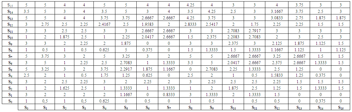 | Table 2. 16×16 Payoff Matrix for Axelrods Values |
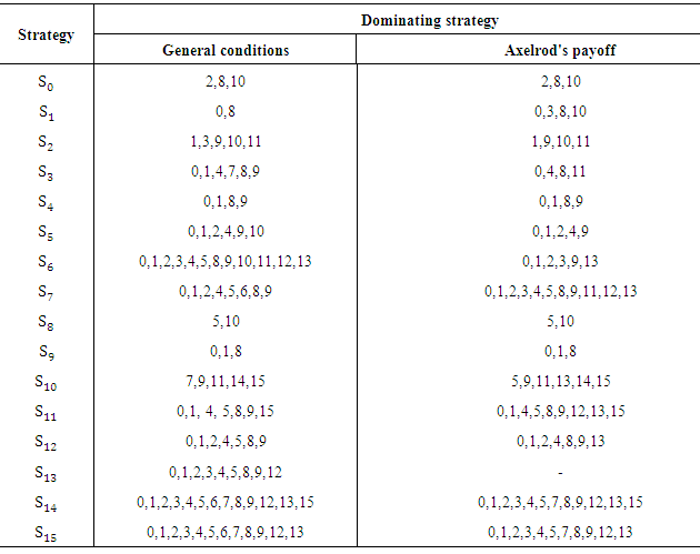
Table 3. Dominating Strategies for General Conditions and Axelrods Values
 |
| |
|
The payoff matrix corresponding to the interaction between strategies  ,
,  and
and  is constructedas follows.
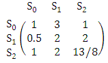 | (7) |
This matrix must be transformed into a system of linear equations.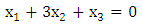 | (8) |
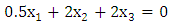 | (9) |
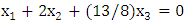 | (10) |
The previous system will be solved together with the following equation to get the equilibrium point.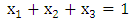 | (11) |
The equilibrium point of the previous system is  .To get the type of the heteroclinic three-cycles (attractors, repellors, centre), the diagonal values of the previous matrix must be transformed to be zeros. This can be achieved by subtracting a constant number from each entry of every column to make the diagonal entry of this column be zero.This algorithm transforms the previous matrix to the following matrix.
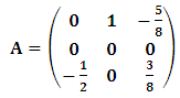 | (12) |
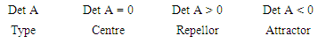 The determinant of the previous example is equal to zero. This means that the type of this heteroclinic three-cycle is centre Figure 2.
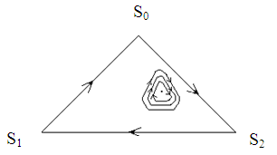 | Figure 2. (S0, S1, S2) centre heteroclinic three-cycle |
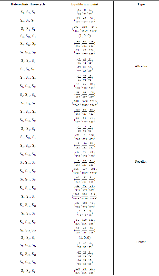
This algorithm will be repeated for every three heteroclinic three-cycles to get all equilibrium points. These equilibrium points will be recorded in Table 4.Table 4. Equilibrium Point and Type of Every Heteroclinic Three-Cycles
 |
| |
|
5. Conclusions
Every row in Table 3 represents strategies which beat Si. The first column represents strategies which beat Si using general conditions. The second column uses Axelrod's values to determine the best strategies. Every column will be studied separately in the following paragraphs.Firstly, it is apparent from Table 3 that at least every strategy is invaded by two strategies for general conditions. It is also noted that S0, S1, S8 and S9 are strong strategies which invade 12 strategies and are invaded by only two strategies for (S1, S8) where (S0, S9) are invaded by three strategies. S14 is invaded by all strategies except S10, S11 and S14 which indicates that it is a very weak strategy.Secondly, what is interesting in this data in column 2 Table 3is that S13 abide in front all the other strategies for Axelrod’s values which means that it is a very strong strategy. S0, S1, S8 and S9 are also strong strategies which invade at least ten strategies. Further analysis showed that there is an inactive strategy S6 which can't invade any strategy. Similarly S14 is outcompeted by the major number of strategies (exactly 12).Thirdly, another important finding is the behavior of S2 and S5 which invade S0 and S8 respectively in both cases. Also these strategies invadea considerable large number of strategies. This in turn means that these strategies act as strong strategies in memory two. S5 (0, 1, 0, 1) which oppose the other player decision in the new state. S2 (0, 0, 1, 0) cooperates only when suckered.Illustration 1The confliction between S8 against S11
 |
| |
|
Fourthly, using mixed strategies for companies example will give better results because there isn't optimum strategy.Finally, there isn't any evolutionary stable strategy so the Table 4 represents every three heteroclinic three-cycle type and equilibrium point.
References
| [1] | Von Neumann, J., Morgenstern, O. (1944) Theory of Games and Economic Behavior. Princeton: Princeton UP, 1953. |
| [2] | Nash, J., Non-cooperative games. Annals of mathematics, 1951: p. 286-295. |
| [3] | Axelrod, R., 7he Evolution of Cooperation. Basic Books, New York. Econornetrica, 1984. 39: p. 383-96. |
| [4] | Aumann, R.J., Survey of repeated games. Essays in game theory and mathematical economics in honor of Oskar Morgenstern, Bibliographisches Institute, Mannheim/ Wien/ Zurich, 1981: p. 11-42. |
| [5] | Rapoport, A. and A.M. Chammah, Prisoner's dilemma: A study in conflict and cooperation. Vol. 165. 1965: University of Michigan press. |
| [6] | Essam, E.-S., The effect of noise and average relatedness between players in iterated games. Applied Mathematics and Computation, 2015. 269: p. 343-350. |
| [7] | Fundenberg, D. and E. Maskin, Evolution and cooperation in noisy repeated games. The American Economic Review, 1990: p. 274-279. |
| [8] | Maskin, F.a., Evolution and repeated games, mimeo, 2007. |
| [9] | E. El-Seidy, Z.K., The perturbed payoff matrix of strictly alternating prisoner's dilemma game. Far Fast J. Appl. Math. 2, 1998. 2: p. 125-146. |
| [10] | Banks, J.S. and R.K. Sundaram, Repeated games, finite automata, and complexity. Games and Economic Behavior, 1990. 2(2): p. 97-117. |
| [11] | Samuelson, L., Evolutionary Games and Equilibrium Selection (Economic Learning and Social Evolution). 1997, MIT Press, Cambridge. |
| [12] | Cressman, R., Evolutionary dynamics and extensive form games. Vol. 5. 2003: MIT Press. |
| [13] | Martin A. Nowak, K.S., Essam El-Sedy, Automata, repeated games and noise. J. Math. Biol., 1995. 33: p. 703-722. |
| [14] | Imhof, L.A., D. Fudenberg, and M.A. Nowak, Tit-for-tat or win-stay, lose-shift? Journal of theoretical biology, 2007. 247(3): p. 574-580. |
| [15] | Rubinstein, A., Finite automata play the repeated prisoner's dilemma. Journal of economic theory, 1986. 39(1): p. 83-96. |
| [16] | Abreu, D. and A. Rubinstein, The structure of Nash equilibrium in repeated games with finite automata. Econometrica: Journal of the Econometric Society, 1988: p. 1259-1281. |
| [17] | Lindgren, K. and M.G. Nordahl, Evolutionary dynamics of spatial games. Physica D: Nonlinear Phenomena, 1994. 75(1): p. 292-309. |
| [18] | Binmore, K.G. and L. Samuelson, Evolutionary stability in repeated games played by finite automata. Journal of economic theory, 1992. 57(2): p. 278-305. |
| [19] | Zagorsky, B.M., et al., Forgiver triumphs in alternating Prisoner's Dilemma. 2013. |
| [20] | Axelrod, R. and W.D. Hamilton, The evolution of cooperation. Science, 1981. 211(4489): p. 1390-1396. |

 Abstract
 Reference
 Full-Text PDF
 Full-text HTML