-
Paper Information
- Paper Submission
-
Journal Information
- About This Journal
- Editorial Board
- Current Issue
- Archive
- Author Guidelines
- Contact Us
Journal of Game Theory
p-ISSN: 2325-0046 e-ISSN: 2325-0054
2013; 2(1): 1-8
doi:10.5923/j.jgt.20130201.01
Bilateral Oligopoly with a Competitive Fringe
 Abstract
 Reference
 Full-Text PDF
 Full-text HTML
Somdeb Lahiri
School of Petroleum Management PD Petroleum University P.O. Raisan Gandhinagar, 382007, Gujarat India
Correspondence to: Somdeb Lahiri, School of Petroleum Management PD Petroleum University P.O. Raisan Gandhinagar, 382007, Gujarat India.
| Email: |  |
Copyright © 2012 Scientific & Academic Publishing. All Rights Reserved.
In this paper we consider a bilateral oligopoly on whose fringe there is a market comprising price taking buyers. The sellers in both markets are the same. The sellers and the buyers in the bilateral oligopoly behave strategically as in a Shapley-Shubik market game. We define the concept of an exact active equilibria and show that if the economy is replicated giving rise to a convergent sequence of (type) symmetric exact active equilibria (i.e. exact active equilibria where all replica of an agent in the original economy choose the same strategy) then the corresponding sequence of price-allocation pairs converge to a competitive equilibrium for the original economy. In a final section we discuss an example of an economy where all buyers have Cobb-Douglas utility functions and show that the concepts introduced in this paper (as also the convergence result) are non-vacuous.
Keywords: Strategic Market Game, Bilateral Oligopoly, Exact Active Equilibrium, Asymptotic Convergence, Competitive Equilibrium
Cite this paper: Somdeb Lahiri, Bilateral Oligopoly with a Competitive Fringe, Journal of Game Theory, Vol. 2 No. 1, 2013, pp. 1-8. doi: 10.5923/j.jgt.20130201.01.
Article Outline
1. Introduction
- The model of strategic market games due to[1],[2] and[3] is based on the assumption of strategic behaviour on the part of buyers and sellers. Unlike Cournot who assumed that buyers are price takers, in strategic market games all the agents are assumed to behave strategically. A particular case of the more general strategic market games is the case of a bilateral oligopoly. In this paper we are concerned with the version of bilateral oligopoly due to[4]. However, we assume that on the fringe of this bilateral oligopoly is a market in which the buyers act as price takers. Thus in our model there are two goods X and Y. X is the numeraire good and also plays the role of money in our model. The other good is Y which is a consumption good. The sellers of Y are initially endowed with Y and no X; the buyers of Y are initially endowed with X and no Y. Ordinarily, with price-taking behaviour on the part of buyers, and all agents caring for both X and Y, our model would be no different from the one proposed by[5] and reproduced in[6] and[7]. In this paper we assume that while buyers care for both X and Y, sellers care only for X and hence are profit maximizers. The sellers are assumed to behave strategically and there are two types of buyers- those who behave strategically and those who are price takers. In the bilateral oligopoly, each seller offers a portion of his initial endowment of Y to the buyers who submit bids in units of X. If the total bids and offers in this market are positive, then the price of Y is determined solely by the ratio of bids to offers. This also determines the price of Y in the market where buyers are price takers. In fact if the price of Y differed on the two markets there would always be scope for arbitrage- someone could buy Y on the market where it is cheaper and sell it for a profit on the market where it is more expensive. The price-taking or competitive buyers express the quantity of Y that they demand at this price. Since the sellers have no use for Y, they offer to the competitive buyers whatever of Y that remains after they have made offers to the strategic buyers. The allocation that is determined after the bids and offers are submitted is as follows. Each seller recovers the value of his offer in the bilateral oligopoly from the strategic buyers. Each strategic buyer gets the quantity of Y that he can purchase with the bid that he has placed in the market for Y. The amount that the sellers offer on the competitive market is distributed among the buyers by using a proportional rule: each buyer obtains an amount of Y that is proportional to the quantity of Y that he demands. Each competitive buyer pays for the Y that he has purchased its value in units of X at the price determined by the bilateral oligopoly. Each seller sells an amount of Y that is proportional to the quantity of Y that he offered on the market and recovers from the competitive market its value in units of X. There are two possibilities in the competitive market: (a) there is excess demand for Y so that the buyers are rationed; or (b) there is excess supply so that each buyer gets whatever of Y he demanded but the sellers sell only a portion of what they offered in the competitive market. We look for an equilibrium in this model where each seller is satisfied with the quantity he offers in the bilateral oligopoly, given the bids and offers of all other strategic players and each strategic buyer is satisfied with his bid, given the bids and offers of all other strategic players. In other words the equilibrium is self enforcing.It turns out that in this model there is a trivial equilibrium: one in which no bids or offers are submitted. Hence we narrow our scope to a particular case of non-trivial equilibrium, i.e. an active equilibrium, one in which all strategic players submit either a positive bid or a positive offer. In this class we further narrow down our interest to only those equilibria where no one is rationed in the competitive market. We call such equilibria, exact active.Our main result says that if the economy is replicated giving rise to a convergent sequence of (type) symmetric exact active equilibria (i.e. exact active equilibria where all replica of an agent in the original economy choose the same strategy) then the corresponding sequence of price-allocation pairs converge to a competitive equilibrium for the original economy. This result is analogous to the asymptotic convergence of Cournot equilibria that is discussed in [8] or[9]. In other words as the number of agents become large, there is at least one sequence of equilibrium price-allocation pairs that approximates a competitive equilibrium, provided there exists a convergent sequence of symmetric exact active equilibria. In a final section we discuss an example of an economy where all buyers have Cobb-Douglas utility functions and show that the concepts introduced in this paper (as also the convergence result) are non-vacuous. Similar analysis for oligopoly in the context of pure exchange economy can be found in[10].Ordinarily the justification for competitive price taking behaviour is the presence of a large number of agents on the same side of the market. However, here we see that even with a small number of agents there is the distinct possibility of price-taking behaviour being sustainable. We do not need an auctioneer to call out the prices on the competitive market. The price is determined by strategic interaction that takes place in a bilateral oligopoly on whose fringe the competitive market is located. Hence this is one case where competitive price formation is possible without either an auctioneer or the assumption of a large number of buyers.Our model should be contrasted with the line of research that originates with the work of Gabszewicz and Vial in[11] where in there is sequential trading between the large traders and the competitive buyers. In this paper we are less concerned with modelling the interaction between buyers and sellers. Our main emphasis is on competitive price formation on the fringe of a bilateral oligopoly. This is an issue that is completely ignored by the literature on imperfect completion irrespective of whether the economy is finite as is usually the case or large as assumed by Shitovitz in[12] and the research that follows from it.
2. The Model
- We consider an economy with two goods X and Y. The players are partitioned into two sides of the market for Y. The set of players is a non-empty finite set H with H = ψ ∪ β where ψ∩β =
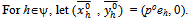
 . Players in ψ are sellers and those in β are buyers of good Y. The initial endowments of the two goods are (eh, 0) if h∈β and (0, eh) if h∈ψ, where eh > 0 for all h∈H. Payments for Y are to be made in units of account of X. X is the numeraire good. It is assumed that the sellers have no use for Y and are only interested in X. Thus sellers maximize profits measured in units of X.An allocation is a list {(xh, yh)}h∈H, such that for all
 ,
,  and
and  . We assume that each player h∈β has a utility function
  such that:(i) uh is continuous on
 .(ii) uh is smooth, strongly increasing (i.e. both first partial derivatives are positive) and strongly concave (i.e. the Hessian matrix is negative definite) on
 .
.
 For
For  , let uh (x,y) denote the marginal rate of substitution
  evaluated at (x,y). It is easy to see that (iv) along with the assumptions that uh is strongly increasing and strongly concave implies that if (x,y) and (x',y') are distinct points belonging to
  with x x' and y ≤ y' then uh (x,y) > uh (x',y'). Further this implication of (iv) implies that the goods X and Y are gross substitutes.The set of buyers β is further divided into two disjoint sets βc and βo, i.e. β = βc∪βo with βc∩βo =
  . The players in Ho = ψ∪βo behave strategically. The buyers in βc behave competitively. In what follows we assume that |ψ| ≥ 2 and |βo|≥ 2 and |βc| ≥ 1. The strategy set of each player h∈Ho is [0,eh].A strategy for h∈ψ denoted qh is the quantity of Y that seller h offers to sell to the buyers in βo and consequently eh – qh is what he offers to sell to the buyers in βc. We write Q to denote
  , and Eψ to denote
  . For h∈ψ, we use Q-h to denote Q -qh and
  to denote
  . A strategy for h∈βo denoted bh is the quantity of X that buyer h bids for Y. We write B to denote the aggregate bid
  and for h∈βo we write
  to denote B – bh.A strategy profile is an array ({qh}h∈ψ ,
  ) where for h∈ψ,qh is a (offer) strategy for seller h, and for h∈βo, bh is a (bidding) strategy for buyer h.
3. The Competitive Buyers
- The procedure that the competitive market adopts is the following. Given a price p > 0, a competitive buyer h∈βc being a price taker solves the following optimization problem:Maximize uh(eh-pyh, yh).Given our assumption on preferences, we know that for all p > 0 and h∈βc there exists a unique
 which solves the problem.Under our assumptions, the function
  is continuously differentiable and
  for all p > 0.Let
  be the function such that for all p > 0,
  . Clearly Yc is continuously differentiable and for all
 .Given a strategy profile ({qh}h∈ψ ,
  ), let Y(p) = Min
 . Since the competitive buyers cannot purchase more than
 , any excess demand requires to be rationed.
4. The Market Game
- Given a strategy profile ({qh}h∈ψ ,
 ) for which BQ > 0, we define a price
 .The allocation {(xh, yh)}h∈H corresponding to the strategy profile ({qh}h∈ψ ,
  ) is the following.For h∈βc:
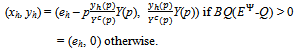 For h∈βo:
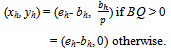 For h∈ψ:
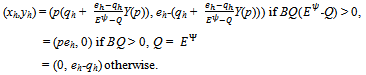 Note that for
 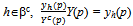 if and only if Y(p) = Yc(p). Otherwise we use the proportional rule to ration the competitive buyers.For h'∈ψ and strategy profile ({qh}h∈ψ ,
  ) we will write xh’({qh}h∈ψ ,
  ) to denote :
 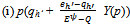 , if
, if  ; (ii)peh’, if BQ > 0,
  ; and (iii) 0, otherwise.For h'∈βo, we shall denote the consumption bundle of h' corresponding to a strategy profile ({qh}h∈ψ ,
  ) by (xh’, yh’)({qh}h∈ψ ,
  )(i.e. (i)
  if BQ > 0; and (ii) 0, otherwise).Given a strategy profile ({qh}h∈ψ ,
  ) and h'∈Ho we shall write:(i) ({q-h’}h∈ψ\{h’} ,
  ) to denote the same strategy profile with the strategy qh’ of h' replaced by
 , provided h'∈ψ.(ii) ({qh}h∈ψ ,
  ) to denote the same strategy profile with the strategy bh’ of h' replaced by
  , provided h'∈βo.An equilibrium is a strategy profile ({qh}h∈ψ ,
  ) such that:(i) For all h'∈ψ: xh’({qh}h∈ψ ,
  ) ≥ xh’({q-h’}h∈ψ ,
  ) whenever
 .(ii) For all h'∈βo: uh’((xh’, yh’)({qh}h∈ψ ,
  ) ≥ uh’((xh’, yh’)({qh}h∈ψ\{h’} ,
  ) for all
 .The following proposition is easily established.Proposition 1: Let ({qh}h∈ψ ,
  ) be a strategy profile such that B = Q = 0. Then ({qh}h∈ψ ,
  ) is an equilibrium. It is called a trivial equilibrium.In view of Proposition 1 we have the following definition.A non-trivial equilibrium is an equilibrium strategy profile ({qh}h∈ψ ,
  ) such that BQ > 0.A non-trivial equilibrium ({qh}h∈ψ ,
  ) is said to be an active equilibrium if:(i) For all h∈ψ: eh > qh > 0.(ii) For all h∈βo: bh > 0.
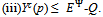 An active equilibrium ({qh}h∈ψ ,
  ) is said to be an exact active equilibrium if
  . Proposition 2: Let ({qh}h∈ψ ,
  ) be an exact active equilibrium. Then
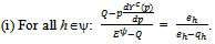 (ii)For all h∈βo:
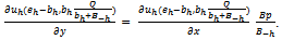 Thus for all h∈βo:
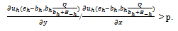
5. Replications of the Basic Economy
- Let us refer to the model that we have discussed above as the basic economy and denote it by E1. We are primarily concerned with the consequences of expanding the basic economy E1. One way to do this is to simultaneously replicate all the agents in the economy a finite number of times. We let IN denote the set of natural numbers. Let kIN. The replicated economy Ek consists of (|ψ|+|β|)k agents, where for each seller h in E1 now there are k sellers each having the same utility function uh and the same initial endowment of Y, eh>0; and for each buyer h in E1 now there are k buyers each having the same utility function uh and the same initial endowment of X, eh > 0. In Ek each seller i{1,…,k} of type h is denoted by (h,i) and each buyer j{1,…,k} of type h is denoted by (h,j). The (offer) strategy q(h,i) of seller (h,i) to the non-competitive buyers belongs to the closed interval[0,eh]. Thus the aggregate supply of good Y to the non-competitive buyers in Ek is
 . Let p > 0 be the price of good Y in terms of good X that the competitive buyers face. Then each competitive buyer (h,j)∈βc{1,2,…,k} solves the following optimization problem:Maximize uh(x,y)
 Under our assumption on preferences there is a unique pair
  which solves this problem. Further x(b,j)(p) + py(b,j)(p) = eh for all p > 0. Thus (x(b,j)(p), y(b,j)(p)) = (xb(p), yh(p)) for all j{1,…,k}. The aggregate quantity of Y demanded by the competitive buyers is
  .Each non-competitive buyer (h,j)∈βo{1,…,k} submits a bid b(h,j)∈[0, eh] in units of X.A strategy profile is a list
  such that for each (h,i)∈ψ{1,…,k},
  is the offer of seller (h,i) and for each (h,j)∈βo{1,…,k},
 is the bid of the non-competitive buyer (h,j).If
 , then the price of Y,
 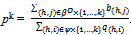 . At strategy profile
  (i) each (h,i)∈ψ{1,…,k} consumes
 (ii) each (h,j) ∈βo{1,…,k} consumes
 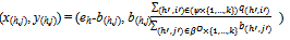 (iii) each (h,j)∈βc{1,…,k} consumes
 An equilibrium for Ek is a strategy profile
 such that:(i) For all (h,i)∈ψ{1,…,k}:

 (ii) For all
 A non-trivial equilibrium for Ek is an equilibrium strategy profile
  such that
 .A non-trivial equilibrium
  is said to be an active equilibrium for Ek if:(i) For all (h,i)∈ψ{1,…,k}: eh > q(h,i) > 0.(ii) For all (h,j)∈βo{1,…,k}: b(h,j) > 0.
 An active equilibrium for
  is said to be an exact active equilibrium (for Ek) if
  .An allocation in Ek is a list {(x(h,i), y(h,i))}(h,i)∈H{1,…,k}, such that for all (h,i)∈H{1,…,k},
  ,
,  and
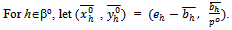
and . For kIN, let
  be a strategy profile in Ek. Let
  for all hψ and
  for all hβo. Thus
  and
and  is a strategy profile for E1.Note that if
  , then the price of Y,
  .For kIN, say that a strategy profile
  is symmetric if (i) for all hψ and
  , and (ii) for all h∈βo and
  . Lemma 1: Let
  be a sequence of strategy profiles in the successive economies {Ek}kIN. Suppose that the corresponding sequence of average strategies
  satisfy
  and converges to some point
  with
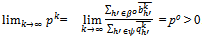
with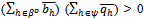 . Then the sequence of prices
  converges to
 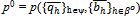 . Moreover, (i) for every sequence
  with
with  for all kIN, and for every sequence of integers {ik}kIN with 1 ≤ ik ≤ k for all kIN, the sequence of prices
  with
with  for all kIN also converges to p0; (ii) for every sequence
  with
with  for all kIN, and for every sequence of integers {ik}kIN with 1 ≤ ik ≤ k for all kIN, the sequence of prices
  with
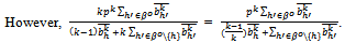
with  for all kIN also converges to p0.
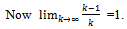
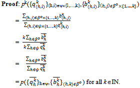 Now since the sequence
 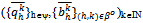 converges to
  with
with , the sequence
 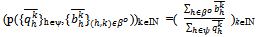 converges to
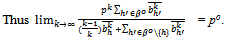
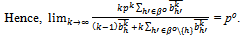
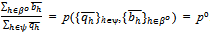 . Thus the sequence of prices
  converges to po.
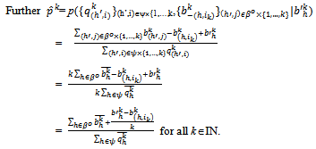 Since the sequences
  and
and  both belong to[0,eh] and are thus bounded
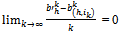 . Thus
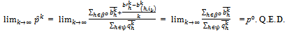
6. Asymptotic Convergence to Competitive Equilibrium
- A price-allocation pair[p; {(xh, yh)}hH] where the latter is a feasible allocation in E1 is said to be competitive if:
 (ii) for all h∈βo: (xh, yh) solves Maximize uh(x’, y’) s.t. x’= eh-py’.
 Theorem 1: Let
 be a sequence of symmetric exact active equilibria in the successive economies {Ek}kIN. Let
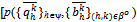 ; {(xk(h,i), yk(h,i))}(h,i)H{1,…,k}] be the price-allocation pair associated to
  . Then for all kIN, hH there exists
  such that for all
  . Assume that the sequence
  converges to some
  with
with . Then the price sequence {pk}kIN where
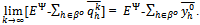
  for all kIN converges to some p0 > 0, and for all
  converges to some
 . Further
 is a competitive equilibrium of the economy E1.Proof: Note that the allocation corresponding to the symmetric exact active equilibrium is the following:

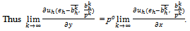
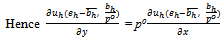
 Now by condition (ii) of Proposition 2, for each (h,i) ∈βo{1,…,k}:
 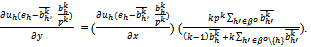 Since
Since converges to some
  with
with ,
, .
.
 Since preferences have been assumed to be C1 on
  and since marginal utililites have been assumed to be unbounded as the consumption of a commodity goes to zero, it follows that for all
  .Since for all h∈βc, yh(.) is C1,
  and
and 

 Also
Also 
 Since for all h∈H we have
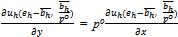 , it must be the case that for all
  solves Maximize uh(x', y') s.t. x'= eh-poy'.Thus
  is a competitive equilibrium. Q.E.D.
7. The Cobb-Douglas Economy
- Suppose ψ = {1,…,N}, βo = {1,…, M} and βc = {1,…, L}. Suppose eh = 1 for all h∈H and there exists γ and η∈(0,1) such that for all
 (i) uh(x, y) = xγ y1-γ whenever h∈βo.(ii) uh(x, y) = xη y1-η whenever h∈βc.
 By the symmetry of the problem within each type of agent, at any active equilibrium ({qh}h∈ψ ,
  ) there exists q, b > 0 such that: (i) for all h∈ψ: qh= q; (ii) for all h∈βo: bh = b.

 At an exact active equilibrium total amount of Y consumed by the buyers is N.
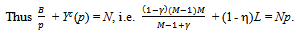
 Note that the profit of each seller is the price p.Further by the symmetry of the problem the offer that each seller submits in the bilateral oligopoly is
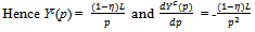
  .We need to verify that no seller can benefit by a unilateral deviation from offering q. There are two possibilities: (a) a unilateral deviation that leads to a decrease in the price of Y, and (b) a unilateral deviation that leads to an increase in the price of Y.Since each seller exhausts his entire supply of Y at an exact active equilibrium, it is not possible for any seller to sell any more. Thus a decrease in price could only lead to a fall in revenue for the sellers and any unilateral deviation by a seller that leads to a decrease in the price that prevails at an exact active equilibrium could not be beneficial for him. Hence we have to see whether a unilateral deviation by a seller that leads to an increase in the price of Y, is beneficial for him. Such a unilateral deviation would involve making an offer less than q. Since such a price rise would lead to a decrease in the quantity of Y demanded in the competitive market, there would be a situation of excess supply in the competitive market and the suppliers would have to be rationed. Since the preference of a competitive consumer is Cobb-Douglas with parameter , each such consumer would spend (1-) on Y and hence the aggregate expenditure of the competitive consumers on Y is (1-)L irrespective of the price. Hence for qh(0, q], the revenue that seller h gets by offering qh when all other sellers offer q is
 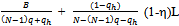 . The derivative of the function
 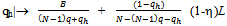 with domain (0,q] is
 The second derivative of this function is
  . Hence this function is concave. If we show that its first derivative at qh = q is non-negative then we are done, since it would imply that the function is maximized at qh = q, and thus there is no unilateral deviation from q that is beneficial to the deviator.


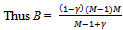
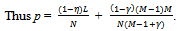
 In view of the above we have the following proposition.Proposition 3: At an exact active equilibrium for the Cobb-Douglas economy the price p of Y is
 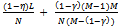 Each non-competitive buyer consumes
 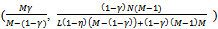 and each competitive buyer consumes
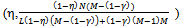 . (a) The price p goes up if N (the number of sellers) remains fixed and either M (the number of non-competitive buyers) or L (the number of competitive buyers) goes up. (b) The price goes down if N goes up with M and L being held fixed. (c) As N goes up (with M and L held fixed) each buyer is better off and each existing seller is worse off. (d) If L goes up (with N and M held fixed) then each existing buyer is worse off and each seller is better off. (e) If M goes up (with L and N held fixed) then again each existing competitive buyer is worse off and each seller is better off. Each non-competitive seller is eventually worse off.Proof: Since (a) to (d) are quite obvious we will prove (e). Suppose M goes up. Consider the price p which is also the profit of a seller. Now
 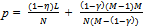 . As M goes up
  increases (towards 1) and M also increases. Thus p goes up and each seller is better off.Consider a competitive buyer. His consumption of X remains fixed at η. His consumption of Y is
 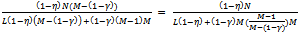 . As before, with an increase in Y,
  increases (towards 1) and M also increases. Thus a competitive buyer’s consumption of Y decreases and each existing competitive buyer is worse off.Consider a non-competitive buyer. As M increases
  decreases (towards 1) and so
  (decreases towards γ). Thus, as M increases his consumption of X decreases.
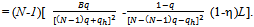
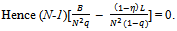
  Now
Now if and only if M(M-1) > (1-γ)γ(1-η)L.Thus a non-competitive buyer’s consumption of Y
 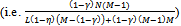 decreases if and only if M(M-1) > (1-γ)γ(1-η)L. Hence as M increases each existing non-competitive buyer is eventually worse off. Q.E.D.In order to compare the consumption of Y between non-competitive and competitive buyers, set M = L and γ = η. Then the consumption bundle of each competitive buyer is
  and the consumption bundle of each non-competitive buyer is
 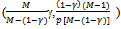 . Since
 , each non-competitive buyer consumes more of X than the competitive buyer. Since
 , each non-competitive buyer consumes less of Y than each competitive buyer.What happens if the above economy is replicated k times, where k is any natural number? In the k-replica of the above economy there are kN sellers, kM non-competitive buyers and kL competitive buyers. As before each seller is a profit maximize and is initially endowed with 1 unit of Y. Each buyer is endowed with 1 unit of X. The utility function of each non-competitive buyer h is uh(x, y) = xγ y1-γ and the utility function of each competitive buyer h’ is uh’(x, y) = xη y1-η.Proposition 4: At an exact active equilibrium for the k-replica of the above Cobb-Douglas economy the price p of Y is
 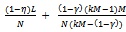 Each non-competitive buyer consumes
 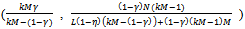 and each competitive buyer consumes
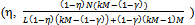 . As k goes to infinity the price converges to
  As k goes to infinity each non-competitive buyer’s consumption bundle converges to
 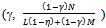 . As k goes to infinity each competitive buyer’s consumption converges to
  .From Proposition 4 it is clear that as k tends to infinity, the sequence of price-allocation pairs converges to the unique competitive equilibrium of the original economy.
 ACKNOWLEDGMENTS
- I would like to thank without implicating Giulio Codognato for his observations and comments on the paper. I deeply indebted to an anonymous referee of this journal for useful comments based on a detailed reading of the manuscript.