1. Introduction

This paper provides a general proof of the existence of pure-strategy Nash equilibria in an n-team sporting contest with heterogeneity of market size and of managerial efficiency among the teams. Since the seminal paper of[21], the Nash equilibrium concept has been used in the analysis of professional team sports. However, there has been no attempt in the literature to provide a general proof of equilibrium existence and uniqueness for economic modeling of team sports. Most papers have been restricted to a two-team league model.¹ Dietl et al.[3] that are considered a more general n-team league model; however, it is based on the assumption that all teams have identical revenue generating potential and cost functions. Thus the sporting contest is symmetric. Moreover, the existing theoretical studies implicitly assume that all team managers/coaches have same managerial skills such as train and motivate individual player to achieve higher levels of playing performance.² Some empirical studies, however, have found evidence that managerial quality and experience is positively related to team and player performance ([10],[18]); in addition, some managers are more efficient than others at transforming a given set of player inputs into team wins ([14],[8]).

These restrictions most probably apply to the Nash equilibrium model in sports because of the difficulty in managing non-identical teams with respect to their market size and/or managerial efficiency by conventional means, which treat the Nash equilibrium as a fixed point of the best response mapping. This entails working in a dimension space equal to the number of teams. In this paper, we adopt an alternative approach introduced in[2], which allows us to work completely with functions of a single variable, considerably simplifying the analysis. In a general asymmetric sporting contest, this paper will prove that under general conditions, there exists a unique non-trivial Nash equilibrium in which at least two teams must be active in equilibrium.

The rest of the paper is organized as follows. Section 2 explains the basic model and the assumptions. In Section 3, we establish the existence of Nash equilibria in an n-team sporting contest. Concluding remarks are presented in Section 4.

2. The Model

We consider a professional sports league consisting of teams where each team independently chooses a level of talent, , to maximize its profits. By assuming a competitive labor market and following the sports economic literature, talent can be hired in the players’ labor market at a constant marginal cost ; hence, the cost function can be written as

(1)

On the revenue side, the season revenue function of a team is defined as

(2)

is total season revenue of team i, w_i is the winning percentage of the team. It is common in the sports economics literature to assume the following.

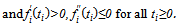
Assumption 1. For all i, the function R_i satisfies and for . Moreover, R_i is twice differentiable and either satisfies and, or there exists a such that if , then ; otherwise, , and elsewhere.

Assumption 1 (A.1 in what follows) is a reflection of the uncertainty of outcome hypothesis ([16],[13]) that consumers in aggregate prefer a close match to one that is unbalanced in favor of one of the teams. Following[15, p. 272], we define the marginal revenue of a win for team i as the market size or drawing potential for the team.³ A particularly well-studied form for R_i is, where represents the market size of team i and characterizes the effect of competitive balance on team revenues.

The win percentage is characterized by the contest success function (CSF). The most widely used functional form in sporting contests is the logit that can be written as

(3)

where.⁴ The factor results from the fact that winning percentages must average to within a league during any one year; that is, . Notice that for the two-team models, the logit CSF (3) does not place a restraint on the teams’ choices. However, for the n-team models this is not the case with the logit CSF (3). More precisely, the winning percentage can be larger than one if a team holds more than per cent of total league talent (with normalization of to one). ⁵To avoid this, we can define the winning percentage as

(4)

As already mentioned in the Introduction, we consider an asymmetric production technology describing the relationship player talent and player performance as follows:

(5)

where is the level of player performance of team i. We call the player-performance production function of team i. It represents the team i’s production technology by which levels of talents are translated into a level of the actual playing performance. We assume that

Assumption 2. For all i the function satisfies the following conditions:

Notice that teams’ production functions do not necessarily have to be identical. For example, a functional of is, where and. This functional form was used by[3] and[6] but assuming identical parameters, i.e., and for all. Since is monotonic, it has a well-defined inverse function, . Then, A.2 implies that

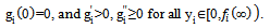(6)

The function times describes the total cost to team of generating the level of performance.

From the player-performance production function (5), the logit CSF (3) and (4), we can define the win percentage of team as follows:

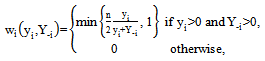(7)

where. Then, the profit of team i is described by

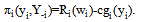(8)

Team i’s original maximization problem is equivalent to the one of maximizing (8) with respect to y_i. This defines a simultaneous-move game and the solution concept we use throughout the paper is that of a pure-strategy Nash equilibrium of this game.⁶

3. Existence Analysis

We can now calculate the best response of team i. Assume first that in order that the other teams do not spend any resources on playing talent. Then, if , the profit is negative in light of A.1, A.2, and (7). If team i sets, the profit becomes zero. Therefore, this game always has a trivial equilibrium point. Our concern is with the non-trivial equilibrium (i.e., ) and thus no further consideration is given to the trivial point.

If, it follows from (8) that we have

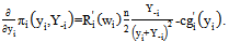(9)

As the second-order condition we get

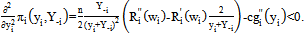(10)

Under A.1 and A.2, the second-order condition (10) is satisfied. Hence, it follows from (9) that given , team i’s best response function is given by

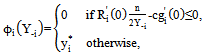(11)

where is the unique solution of the strictly monotonic equation

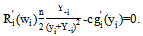(12)

Observe that due to A.1 and A.2 the left-hand side of (12) strictly decreases and is continuous in and positive at; therefore there is a unique solution. It is well known that a strategy profile is an equilibrium if and only if for all i, is the best response with fixed values of .

Further, we can rewrite the best responses of the teams in terms of aggregate player performance, which we will denote by . From (11), we have

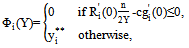(13)

where solves equation

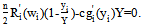(14)

Note that in the second case of (13), the left-hand side of (14) is positive at and strictly decreasing, because it has a negative derivative given by

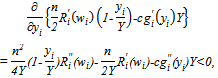where the sign comes from A.1 and A.2. Therefore there is a unique solution of equation (14), which is a continuously differentiable function of by the implicit function theorem. Following[23, p. 91], we call the inclusive reaction function of team i, which is proposed by[19].

Rather than use the inclusive reaction function directly, we will examine properties of player i’s share function, which is proposed by[2]. It can be readily checked that Nash equilibrium values of Y occur where the aggregate share function equals unity. That is, . Given, the corresponding equilibrium is found by multiplying by each team’s share evaluated at:. This result enables us to prove the existence of a unique equilibrium by demonstrating that the aggregate share is equal to one at a single value of Y. We can now define a share function for each team and denote team i’s share value by

Lemma 1. Under A.1 and A.2, there exists a share function: . satisfies

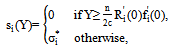(15)

where is the unique solution of

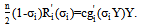(16)

Proof. Using we can rewrite (14) as (16). Recall that a team’s winning percentage in (7) is determined by the ratio of its performance to aggregate performance in the league. Therefore, team i’s revenue can be written as a function of .

Let us denote the left-hand side of (16) by and the right-hand side by. An intersection of these two functions, if any, which is a solution of (16), determines share values. The function is strictly decreasing if and only if A.1 holds. It is bounded from above (i.e., ) and below (i.e., ). In contrast, the function is non-decreasing in due to A.2. It is bounded from above (i.e., ) and below (i.e., ). Thus, we may conclude that there is a unique share value for any which is zero if and only if. The proof is completed by observing that.

The following lemma gives the crucial qualitative properties of the share function derived under A.1 and A.2.

Lemma 2. Under A.1 and A.2, the share function has the following properties:

1. is continuous,

2. , and

3. is strictly decreasing where positive.

Proof. First, note that the shares are continuous (indeed differentiable where positive) by the implicit function theorem, establishing Part 1. Second, since is finite, letting in both sides of (16) demonstrates that the share must approach one as Y approaches zero, giving Part 2. To justify Part 3, we investigate the slope of . The total differential of (16) has the following form:

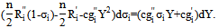We can then express the slope of as follows:

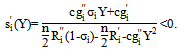The inequality follows since the denominator is negative by A.1 and the numerator is positive by A.2. We may deduce that the positive shares are strictly decreasing in Y, establishing Part 3.

This completes the proof.

It follows from Lemma 2 that the aggregate share function is continuous, exceeds 1 for small enough Y, is less than 1 for large enough Y, and is strictly decreasing when positive. Therefore, the equilibrium value is unique. Finally, recall that a unique implies a unique strategy profile , and we have the following result.

Theorem 1. Under A.1 and A.2, the sporting contest has a unique non-trivial Nash equilibrium in pure strategies.

Notice that for all team i and any fixed value of , the solution always gives zero profit for this team. Therefore, at the best response, team i’s profits must not be negative. Hence, under A.1 and A.2, each team enjoys nonnegative profits at the equilibrium.

4. Conclusions

This study has proven that under general conditions, a unique non-trivial Nash equilibrium exists in a contest model of an n-team sports league with different drawing potentials and different managerial skills among the teams. Over the past few years, the Nash equilibrium concept has been used in the analysis of professional team sports. A particularly great deal of attention has been focused on revenue sharing’s effects on competitive balance. However, when the number of teams exceeds by two, revenue sharing’s effects on the competitive balance are not clearly described. This study applies the share function approach to a general n-team professional sports model, an approach that avoids the dimensionality problem associated with the best response function approach. We believe that the present paper may serve as a basis for further research on the effects of competitive-balance rules, such as revenue sharing and salary caps.

Notes

1. An excellent review of these studies is provided by[11].

2. An interpretation of the same skill is that as noted by[9], managers are nothing more than the principal clerks that make little difference in team performance. However, for several reasons, the result of Horowitz is not entirely convincing. See[17] for details.

3. Burger and Walters[1] and[12] empirically found that the marginal revenue of the win of a large-market team is larger than that of a small one in Major League Baseball.

4. The logit CSF is explicitly adopted in the seminal work of[4]. See also the excellent survey by[20].

5. Groot[7, pp. 97-100] has expressed the season winning percentage as follows: . Although this equation gives the correct relationship between winning percentage and team quality, it considerably complicates the derivative of the marginal product of talent. We therefore choose the simple approximation of the winning percentage (3).

6. It is occasionally assumed that the total supply of talent is fixed in the analysis of sports leagues. Authors who have made this assumption have used a non-Nash conjecture to reflect this scarcity in each team’s first-order condition ([5],[22]). In this case and for a two-team we have. Indeed, although opinion is divided among sports economists on this subject, we use the Nash conjecture in this paper (see e.g.,[11]).

ACKNOWLEDGEMENTS

The earlier version of this paper was presented at the 2012 Spring Meeting of the Japanese Economic Association, Hokkaido University, Hokkaido, Japan, June 23-24, 2012. The author wishes to thank participants, Professor Akio Matsumoto of Chuo University, Professor Yoshihiro Yoshida of Seikei University, and a referee and an associate editor of this journal for their kind advices. The usual disclaimer applies.