-
Paper Information
- Previous Paper
- Paper Submission
-
Journal Information
- About This Journal
- Editorial Board
- Current Issue
- Archive
- Author Guidelines
- Contact Us
Journal of Game Theory
2012; 1(4): 25-28
doi: 10.5923/j.jgt.20120104.02
Endogenous Leadership in a Labor-Managed Duopoly
 Abstract
 Reference
 Full-Text PDF
 Full-Text HTML
Kazuhiro Ohnishi
Institute for Basic Economic Science, Minoo, Osaka 562-0044, Japan
Correspondence to: Kazuhiro Ohnishi , Institute for Basic Economic Science, Minoo, Osaka 562-0044, Japan.
| Email: |  |
Copyright © 2012 Scientific & Academic Publishing. All Rights Reserved.
This paper examines a quantity-setting model in which two labor-managed firms compete against each other. The paper considers the following situation. Each labor-managed firm must choose output either in period one or in period two. If the labor-managed firms decide to choose output in the same period, a simultaneously move game occurs, whereas if the labor-managed firms decide to choose output in different periods, a sequential move game arises. The paper demonstrates that there is no equilibrium where the labor-managed firms choose output in the same period.
Keywords: Quantity-Setting Model, Labor-Managed Duopoly, Endogenous Leadership
1. Introduction
- Hamilton and Slutsky[1] consider the novel issue of endogenous timing in two-player games, with important modeling implications for several models in industrial economics. In a preplay stage, players decide whether to select actions in the basic game at the first opportunity or to wait until they observe their rivals’ first period actions. In one extended game, players first decide when to select actions without committing to actions in the basic game. The equilibrium has a simultaneous play subgame unless payoffs in a sequential play subgame Pareto dominate those payoffs. In another extended game, deciding to select at the first turn requires committing to an action. They show that both sequential play outcomes are the equilibria only in undominated strategies. In addition, Yang et al.[2] compare Bertrand and Cournot equilibria in a differentiated product duopoly under endogenous timing with observable delay, and demonstrate that endogenous timing leads to two sequential play with both leader-follower configurations in Bertrand, but simultaneous play in Cournot. There are many further studies (see, for example,[3-14]). However, these studies are models with profit-maximizing capitalist firms and do not include labor-managed firms.Therefore, we examine an endogenous timing in labor-managed duopoly competition. The pioneering work on a theoretical model of a labor-managed firm was conducted by[15]. Since then, many economists have studied the behaviors of labor-managed firms (see, for example,[16-31]) (see also[32-35] for excellent surveys).Lambertini[36] considers a mixed duopoly where a profit-maximizing and a labor-managed firm compete either in prices or in quantities and shows that if firms can choose the timing of moves before competing in the relevant market variable, the Bertrand game yields multiple equilibria, while the Cournot game has a unique subgame perfect equilibrium with the profit-maximizing firm in the leader’s role and the labor-managed firm in the follower’s role. Lambertini[36] considers mixed market competition with profit-maximizing and labor-managed firms, while we investigate pure market competition with labor-managed firms.We examine a Cournot model in which two labor-managed firms compete against each other. The game is as follows. Each labor-managed firm must choose output either in period one or in period two. If the labor-managed firms decide to choose output in the same period, a simultaneously move game occurs, whereas if the labor-managed firms decide to choose output in different periods, a sequential move game arises.The purpose of this study is to present the equilibrium of endogenous timing Cournot competition where two labor-managed firms compete against each other.The remainder of this paper is organized as follows. In Section 2, we describe the model. In Section 3, we discuss the equilibrium of the model. Finally, Section 4 concludes the paper.
2. The Model
- Let us consider a market with two labor-managed firms, firm A and firm B. In the remainder of this paper, subscripts A and B denote firm A and firm B, respectively. In addition, when i and j are used to refer to firms in an expression, they should be understand to refer to A and B with
 . The market price is determined by the inverse demand function
 , where
 . We assume that
  and
and  . This assumption includes linear and constant elasticity demand functions such as
  ,
,  .1Firm i’s income per worker is given by
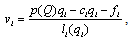 | (1) |
 denotes firm i’s capital cost for each unit of output,
  is firm i’s fixed cost, and
  is the number of workers in firm i. We assume that
  and
and  . Each firm chooses
  in order to maximize (1).The timing of the game is as follows. In period 0, each firm simultaneously and independently chooses
  , where
  indicates when to decide the non-negative output
  . That is,
  implies that firm i decides in period 1, and
  implies that it decides in period 2. At the end of period 0, each firm observes
  and
and  . In period 1, firm i choosing
  selects its output
  in this period. In period 2, firm i choosing
  selects its output
  in this period. At the end of the game, the market opens and each firm sells its output
  .
.3. Equilibrium
- In this section, we discuss the equilibrium of the model described in the previous section. We use subgame perfection as the equilibrium concept. We restrict our attention to pure strategy equilibria.First, we derive the reaction functions in quantities. The equilibrium occurs where each firm maximizes its objective with respect to its own output level, given the output level of its rival. Firm i’s reaction function is defined by
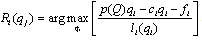 | (2) |
 is upward sloping.Proof. Firm i aims to maximize its income per worker with respect to its own output level, given the output level of firm j. The equilibrium must satisfy the following conditions: The first-order condition for firm i is
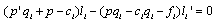 | (3) |
 | (4) |
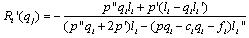 | (5) |
 is a function of
  and
and  , so that
  is positive. Q.E.D.Both firms’ reaction curves are drawn in Figure 1, where
  is firm i’s reaction curve. Both firms’ reaction curves are upward sloping. This means that both firms treat quantities as strategic complements2. The reaction curves cross twice; that is, there are two Cournot equilibria. Only point C is a stable Cournot equilibrium, since in point D firm B’s reaction curve crosses firm A’s from above3. It is clear that each firm’s income per worker is higher at C than at D. In the remainder of this paper, we will not consider the unstable Cournot equilibrium D.
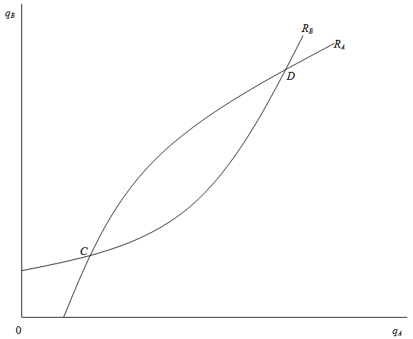 | Figure 1. Reaction curves in quantity space |
 , and firm j selects
  after observing
  . Firm i maximizes
  with respect to
  We present the following two lemmas, where the superscripts L, F, and C denote the Stackelberg leader outcome, the Stackelberg follower outcome, and the Cournot-Nash outcome, respectively.Lemma 2. (i)
  and (ii)
  .Proof. (i) If firm i is the Stackelberg leader, then it maximizes
  with respect to
  . Therefore, firm i’s Stackelberg leader output satisfies the first-order condition:Lemma 1 states that
  is positive. Since
  and
and  ,
,  must be positive to satisfy (6).(ii) Lemma 1 shows that
  is strictly positive. Lemma 2 (i) means that firm j’s Stackelberg leader output is smaller than its Cournot output. Thus Lemma 2 (ii) follows. Q.E.D.Lemma 3. (i)
  and (ii)
  .Proof. (i) Since the Stackelberg leader maximizes its income per worker and can choose
  , we obtain
  . Lemma 2 (i) states
  . Thus Lemma 3 (i) is derived.(ii) Since
  , decreasing
  increases
  given
given  , and thus Lemma 3 (ii) follows. Q.E.D.These lemmas indicate that each firm has an incentive to decrease its output.We now present the equilibrium of the observable delay game formulated in Section 2.Proposition 1. The game has two pure-strategy Nash equilibria: (1, 2) with payoffs
  and (2, 1) with payoffs
  .Proof. In period 0, each firm simultaneously and independently chooses
  . At the end of period 0, each firm observes tA and tB. In period 1, firm i choosing
  selects its output in this period. In period 2, firm i choosing
  selects its output in this period. At the end of the game, the market opens and each firm’s income per worker is decided. Our equilibrium concept is subgame perfection, and all information in the model is common knowledge. Hence, we can consider the following payoff matrix:
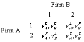 Thus, the proposition follows from Lemma 3. Q.E.D.Proposition 1 means that each firm is either a leader or a follower.
4. Conclusions
- We have examined endogenous timing in a Cournot duopoly where two labor-managed firms compete against each other. There are two production periods, and the labor-managed firms simultaneously and independently announce in which period they will choose their outputs. If the labor-managed firms decide to choose output in the same period, a simultaneously move game occurs, whereas if the labor-managed firms decide to choose output in different periods, a sequential move game arises. We have shown that there is no equilibrium where the labor-managed firms choose output in the same period. As a result, we have found that each firm may play the role of Stackelberg leader.
Notes
- 1. See, for example,[37].2. The concept of strategic complements is introduced by[38].3. For this point, see[26].