Germán Coloma
CEMA University, Av. Cordoba 374, Buenos Aires, C1054AAP, Argentina
Correspondence to: Germán Coloma , CEMA University, Av. Cordoba 374, Buenos Aires, C1054AAP, Argentina.
| Email: |  |
Copyright © 2012 Scientific & Academic Publishing. All Rights Reserved.
Abstract
This paper presents a model of the penalty-kick game between a soccer goalkeeper and a kicker, in which there is uncertainty about the kicker’s type (and there are two possible types of kicker). Both the goalkeeper and the kicker can choose among three different strategies (right, left and center). To find a solution for this game we use the concept of Bayesian equilibrium. Comparing this equilibrium with the corresponding complete-information Nash equilibria, we find that in all cases the expected scoring probability increases (so that, on average, the goalkeeper is worse off under incomplete information). The model is also useful to explain why it could be optimal for a goalkeeper never to choose the center of the goal (although at the same time there are some kickers who always chose to shoot to the center).
Keywords:
Soccer Penalty Kicks, Scoring Probabilities, Bayesian Equilibrium, Incomplete Information
1. Introduction
The penalty-kick game, in which a soccer goalkeeper and a kicker face each other, has become an important example in the applied game-theory literature to analyzemixed-strategy Nash equilibria. The reason of this importance probably has to do with the fact that it is a game whose solution generates a clear theoretical prediction and, at the same time, it is relatively easy to gather data about actual outcomes of the game.All the game-theoretic literature that we know about penalty kicks analyzes this situation as a game of complete information, i.e., as a game in which the two players know the characteristics of each other, and hence they know the expected payoffs that they will receive in the different strategy profiles of the game. There is a good reason for this assumption, which is the idea that goalkeepers and kickers in a professional soccer league are usually well-known players whose main characteristics are recognized by theiropponents, and those characteristics are precisely the ones that define the parameters which establish the expected payoff of the penalty-kick game. Complete-information games, moreover, are also easier to solve and, perhaps more importantly, are easier to test empirically. This ease is probably the best explanation for the success of the penalty-kick game as a prominent example in the game-theoretic literature.Not all soccer penalty kicks, however, are shot in situations in which it is reasonable to assume complete information. In many cases, especially in amateur matches and in matches between teams that belong to different leagues, it is possible that players do not know each other and,therefore, are uncertain about several important characteristics that may influence the outcome of the game. It is also possible that the kicker (and, less usually, the goalkeeper) is a player who is not the “typical choice” in his team, because he is out of the match or because the team has decided to change him due to a poor past performance. Moreover, as penalty kicks are sometimes used as tie-breakers in some tournaments, and this requires that several players from each team shoot penalty kicks, it is possible that some of the designated kickers do not usually shoot penalty kicks in professional matches. This may generate a situation in which the goalkeeper is uncertain about some of the kicker’s relevant characteristics, changing the game into one with incomplete information.When we have to analyze a game with incomplete information, the main solution concept for games with complete information (i.e., Nash equilibrium) is usually unavailable. Since the seminal contribution by Harsanyi[7], however, we have an alternative concept to apply in these cases, which is the so-called “Bayesian equilibrium”. This equilibrium relies on the idea that, under incomplete information, players typically have data about the probabilities of their opponents’ characteristics, and this allows them to figure out which are the different “types” of opponents that they may face and the probability associated to each type. With that information we can build an equilibrium in which each player’s type plays his best response to their opponents’ strategies, taking into account the probability of facing each opponent’s type.In this paper we will develop a model of a penalty-kick game in which there is a single type of goalkeeper and two types of kickers. This is consistent with several results that appear in the literature, in the sense that professional goalkeepers are basically homogeneous in theircharacteristics as penalty-kick savers, and that the main variation that we observe comes from the kickers’ side.In the next section of this paper we will review the main literature about the problem. After that, in section 3 we will present a model in which we will allow for uncertainty about one of the parameters that define the scoring probabilities of the penalty-kick game. This change, together with the inclusion of an additional parameter that defines the probability distribution of the kicker’s types, will generate a new game in which the kicker plays knowing the goalkeeper’s characteristics but the goalkeeper plays against an uncertain opponent (who may be of two different types). We will also compare the solution of this game with their complete-information counterparts, i.e., with the Nash equilibria of the games in which the goalkeeper alternatively faces each of the kicker’s types.In the fourth section of the paper, we will include a few numerical illustrations of the model. One of them will be a theoretical example in which we will explore the equilibria when the distribution of kicker’s types change. Following that, we will develop an empirical illustration based on data from previous studies about the penalty-kick game. Finally, the fifth section will be devoted to the conclusions of the whole paper.
2. Review of the Literature
The seminal work about the penalty-kick game is Chiappori, Levitt and Groseclose[3]. In that paper, the authors develop a model of a game between a soccer goalkeeper and a kicker in which each player can choose among three different strategies (left, right and center), and find that the complete-information Nash equilibrium of that game is unique. They also find, however, that depending on the scoring probability associated to shooting to the center of the goal, that equilibrium can be of two classes. If that scoring probability is relatively low, then the equilibrium is what they call a “restricted-randomization equilibrium”, in which both the goalkeeper and the kicker randomize between left and right, but they never choose the center. If conversely, the scoring probability of shooting to the center of the goal (when the goalkeeper chooses one of his sides) is relatively large, then we find a “general-randomization equilibrium” (in which both the goalkeeper and the kicker randomize among left, right and center).Different types of kickers also change the Nash equilibrium in other versions of the penalty-kick game. In Palacios-Huerta[10], for example, both the goalkeeper and the kicker choose between two strategies (left and right), but the equilibrium mixed strategies are functions of the scoring probabilities of the four possible strategy profiles. Changing one of these parameters, therefore, changes the equilibrium; and playing a strategy that is an equilibrium one for a certain set of parameters when the set of parameters is different, consequently, implies that the other player’s best response is a pure strategy and not a mixed one.Another example of the penalty-kick game literature is Jabbour and Minquet[8], where there is an additional strategy dimension (the height of the kicker’s shot), and shooting high to one of the sides (left or right) assures the kicker a certain scoring probability (because the goalkeeper cannot save the shot, and his only hope is that the kicker shoots outside the goal). In this case we also have two classes of Nash equilibrium, which depend on the scoring probability of shooting high: if this probability is relatively small, then the kicker will randomize between shooting right-low or left-low (but he will never shoot high); if it is large, then the kicker will strictly prefer to shoot high, and he will always choose one of the sides.The use of game-theoretic models to analyze the interaction among soccer players has also gone beyond the penalty-kick situation. In Moschini[9], for example, there is a version of a similar game applied to a situation where a kicker has to choose between shooting at the near post or the far post of a goalkeeper, and the goalkeeper has to choose a certain position in the goal line (closer to the near post or to the far post). The Nash equilibrium of this game is also constituted by mixed strategies, so the kicker randomizes between the near post and the far post, and the goalkeeper chooses an intermediate position between the two posts.Different kicker’s strategies have also been considered to analyze the scoring probability in penalty kick and other shooting situations during a soccer match. In Pollard, Ensum and Taylor[11], for example, the authors estimate that probability as a function of the distance between the kicker and the goalkeeper, the angle from the goalpost and, in cases where the shots occur during a match, the space from the nearest opponent at the time of the shot.General kicker’s ability is also another factor that has been considered as a possible determinant of the scoring probability in a penalty-kick situation, which also has implications in the strategy choice. This is basically the point made by Bauman, Friehe and Wedow[2], who develop and test a game-theoretic model in which they seek to explain differences in mixed strategies associated with different kicker’s types and the relative performance of those types. Using that model they find, for example, that more able kickers show a higher degree of specialization, i.e., they tend to choose a particular side more often. Following a similar line, Coloma[4] has analyzed the difference in scoring probabilities induced by restricted-randomization and general-randomization equilibria, using the same data on which[3] is based.The literature on penalty kicks has also developed a branch which has incorporated elements of psychological economics. Dohmen[6], for example, has analyzed the idea that the presence of spectators generates some “incentive detrimental effects” that reduce the scoring probability in a penalty-kick situation. In a similar line, Savage and Torgler[12] find that extreme pressure can have either positive or negative impacts on the individual kicker’s performance, basically depending on the relative advantage of the kicker’s team in the situation in which he shoots.The most interesting contribution of the psychological economics’ literature to the problem analyzed in this paper, however, is probably the one by Bar-Eli et al.[1]. In their article, these authors point out a problem of the complete-information version of the penalty-kick game, concerning the relatively small frequency that goalkeepers choose to stay in the center of the goal. This phenomenon is seen as a weakness of the game-theoretic approach to penalty kicks, and it is explained using an alternative approach, called “norm theory”. The essence of that approach is that goalkeepers are not actually minimizing an expected scoring probability but following a social norm that prescribes a certain action (jumping to the right or to the left) instead of a situation of “inaction” (i.e., staying in the center of the goal).All the contributions of both the game-theoretic and the psychological economics’ literature, however, are based on models that rely on complete information. We will see that when we abandon that complete-information assumption, even in a relatively simple fashion, we find new ways of explaining some phenomena regarding both the goalkeeper’s and the kicker’s strategies in a penalty-kick situation, and those ways are able to conciliate some results that come from the game-theoretic literature and some others that have been pointed out by alternative approaches.
3. The Model
3.1. Complete Information
Following the notation that appears in Coloma[4], we will build a game in which the kicker has to choose among his natural side (the goalkeeper’s right, if the kicker is right-footed, or the goalkeeper’s left, if the kicker is left-footed), his opposite side (the goalkeeper’s left, if the kicker is right-footed, or the goalkeeper’s right, if the kicker is left-footed) and the center of the goal. Similarly, the goalkeeper has to choose among the kicker’s natural side (NS), the kicker’s opposite side (OS) and the center of the goal (C)1. The probability of scoring if both the kicker and the goalkeeper choose NS is PN, while the probability of scoring if both the kicker and the goalkeeper choose OS is PO. If the kicker chooses NS but the goalkeeper chooses OS or C, then the scoring probability is πN, while the scoring probability in the case that the goalkeeper chooses NS and the kicker chooses OS or C is πO. If the kicker chooses C and the goalkeeper chooses NS or OS, then the scoring probability is equal to μ, while we will assume that the scoring probability is equal to zero if both the goalkeeper and the kicker choose C.As this is a constant-sum game in which the kicker wins if he scores and the goalkeeper wins if the kicker does not score, then the kicker’s expected payoff can be associated to the scoring probability and the goalkeeper’s expected payoff can be associated to the complement of that probability. As it is a simultaneous game, then the kicker’s strategy space consists of three strategies (NS, C and OS) and the goalkeeper’s strategy space also consists of three strategies (NS, C and OS).Both the theoretical and the empirical literature agree that the scoring probabilities of the penalty-kick game have to be defined so that “πN ≥ πO > μ > PN > PO > 0”, and these conditions guarantee that the Nash equilibrium of the complete-information version of the game is a mixed-strategy one, in which both the kicker and the goalkeeper choose NS, C and OS with certain probabilities. Let us use the letters n and c to define the probabilities with which the kicker chooses NS and C (so that the probability that he chooses OS is “1-n-c”). Correspondingly, let us use the letters ν and γ to define the probabilities with which the goalkeeper chooses NS and C (so that the probability that he chooses OS is “1-ν-γ”).Let us now assume that there are two types of kicker (kicker 1 and kicker 2) and a single type of goalkeeper. Those kickers are characterized by having different values for the parameter μ, such that “μ1 < μ2”. The corresponding probability matrix, therefore, is the one that appears on table 1.| Table 1. Scoring-probability matrix |
| | | | Goalkeeper | | | | NS | C | OS | | Kicker 1 | NS | PN | πN | πN | | C | μ1 | 0 | μ1 | | OS | πO | πO | PO | | Kicker 2 | NS | PN | πN | πN | | C | μ2 | 0 | μ2 | | OS | πO | πO | PO |
|
|
Let us assume, moreover, that the values of μ1 and μ2 are such that: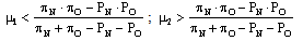 | (1) . |
Following Chiappori, Levitt and Groseclose[3], we know that in this case the corresponding complete-information Nash equilibria occur when it holds that (game 1):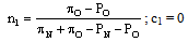 | (2) ; |
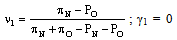 | (3) ; |
and when it holds that (game 2):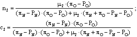 | (4) ; |
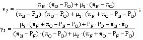 | (5) ; |
where n1, c1, ν1 and γ1 define the strategies that correspond to game 1 (i.e., to the game between the goalkeeper and kicker 1) and n2, c2, ν2 and γ2 define the strategies that correspond to game 2 (i.e., to the game between the goalkeeper and kicker 2).As we see, the fact that μ1 is a relatively small number induces kicker 1 not to choose C in any circumstance (i.e., it makes C a dominated strategy for kicker 1). Knowing that, the goalkeeper never chooses C, either, when facing kicker 1. Conversely, as μ2 is relatively large, kicker 2 is willing to choose C with some positive probability. Knowing that, the goalkeeper sometimes chooses C when facing kicker 2. Following the terminology of[3], we will say that the Nash equilibrium of the game between kicker 1 and the goalkeeper is a “restricted-randomization equilibrium”, while the Nash equilibrium of the game between kicker 2 and the goalkeeper is a “general-randomization equilibrium”.
3.2. Incomplete Information
Let us now turn to an incomplete-information case, in which the goalkeeper does not know if he is facing kicker 1 or kicker 2, but the kicker knows his type (and also the unique goalkeeper’s type). Let us assume that there is a probability θ that the goalkeeper faces kicker 1, and a probability 1-θ that he faces kicker 2. In that case we have to look for a Bayesian equilibrium, in which the goalkeeper chooses a single strategy and each of the possible kickers chooses his own strategy.One possible Bayesian equilibrium for this situation (case A) occurs when the goalkeeper chooses the same strategy that he would choose in a complete-information setting in which he were facing kicker 1 (i.e., νA > 0, γA = 0). Given that, kicker 1 is indifferent between choosing NS and OS, and kicker 2 is strictly better-off by choosing C, provided that the goalkeeper never chooses C in his equilibrium strategy. All these results can be stated as follows: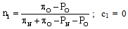 | (6) ; |
 | (7) ; |
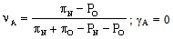 | (8) . |
Another possible Bayesian equilibrium (case B) occurs when the goalkeeper chooses the same strategy that he would choose in a complete-information setting in which he were facing kicker 2 (i.e., νB > 0, γB > 0). Given that, kicker 2 is indifferent between choosing NS, OS or C, and kicker 1 is indifferent between choosing NS or OS2 This implies that: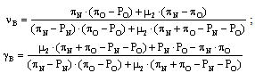 | (9) ; |
 | (10) ; |
 | (11) ; |
where SP1 is the expected scoring probability for kicker 1 and SP2 is the expected scoring probability for kicker 2.The values for n1 and n2 in this Bayesian equilibrium, however, are indeterminate, since what we need is that, on average, they equate the value that n2 has in the corresponding complete-information Nash equilibrium. The equilibrium value for c2, conversely, is a function of the parameter θ. Indeed: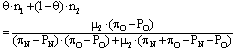 | (12) ; |
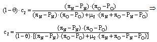 | (13) |
For these strategy profiles to be Bayesian equilibria, however, some additional conditions have to be fulfilled. Under case A, for example, we need that the goalkeeper be indifferent between choosing NS and OS, and strictly better-off by choosing any of those strategies than by choosing C. Let us now define the corresponding expected scoring probabilities induced by the three possible goalkeeper strategies (NS, OS and C) in the following way: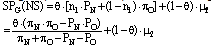 | (14) |
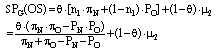 | (15) |
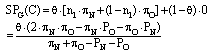 | (16) |
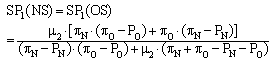
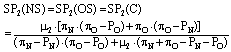
As we see, the equilibrium values found for n1 and c2 imply that in this case SPG(NS) and SPG(OS) are equal, so the goalkeeper is actually indifferent between choosing NS and OS. We will also need that, in this equilibrium, SPG(NS) and SPG(OS) are greater than SPG(C), but this only occurs for a set of values of the parameter θ, as the following proposition shows.Proposition 1: If the Bayesian equilibrium of the case A incomplete-information game exists, then it should hold that “θ > μ2∙(πN+πO-PN-PO)/[(πN-PN)∙(πO-PO)+μ2∙(πN+πO-PN-PO)]”.Proof: Under the Bayesian equilibrium of case A, the goalkeeper should strictly prefer to play both NS and OS with a positive probability, instead of C. Therefore it should hold that: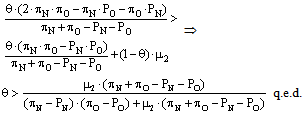 On the other hand, for a case B equilibrium to exist, it is important that n1, n2 and c2 take some values that are not inconsistent with their status as probability values. In particular, we need that c2 is not greater than one, and this also occurs for a particular set of values of the parameter θ. This is the theme of proposition 2.Proposition 2: If the Bayesian equilibrium of the case B incomplete-information game exists, then it should hold that “θ < μ2∙(πN+πO-PN-PO)/[(πN-PN)∙(πO-PO)+μ2∙(πN+πO-PN-PO)]”.Proof: Under the Bayesian equilibrium of case B, kicker 2 should choose C with a certain probability (c2) that guarantees that the goalkeeper is indifferent between choosing NS, OS and C. But this can only be feasible if the required equilibrium value for c2 is less than one. Therefore it should hold that:
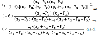 Note that propositions 1 and 2 imply that case A and case B equilibria cannot exist at the same time. Indeed, for any particular value of θ, only one of these equilibria can occur, being case A equilibrium the chosen one when θ is relatively large, and case B equilibrium the chosen one when θ is relatively small.Another set of restrictions on parameter θ can be found if we analyze the possible values of n1 and n2 under a case B equilibrium3. Recall that, from equation 12, we know that n1 and n2 have to be such that, on average, they are equal to μ2∙(πO- PO)/[(πN-PN)∙(πO-PO)+μ2∙(πN+πO-PN-PO)]. But the possible combinations of n1 and n2 that satisfy that equation are also limited by the conditions that “0 ≤ n1 ≤ 1”, and “0 ≤ n2 ≤ 1-c2”. In the particular cases where one of these constraints holds as an equality, then the other strategy coefficient adopts a determinate value. But this value is also constrained by some restrictions, and this imposes additional limits on the possible values for the parameter θ.
3.3. Average Scoring Probabilities
An additional group of results that we can find using our incomplete-information model has to do with the idea that the average scoring probabilities are higher under incomplete information than under complete information. In order to show this, it is useful to prove first (lemma 1) that under complete information the expected scoring probability is smaller for game 1 than for game 2. This has to do with the fact that we are assuming that “μ1 < μ2” (and all the other parameters are the same for the two types of kicker).Lemma 1: Under complete information, the expected scoring probability for kicker 1 is smaller than the expected scoring probability for kicker 2.Proof: Substituting the complete-information equilibrium values of ν1, ν2 and γ2 into the expected scoring probabilities of kickers 1 and 2 when they either choose NS, OS or C, we can write that: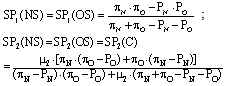 If we assumed that “SP1(CI) > SP2(CI)”, then it should hold that:
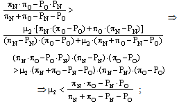 but this is a contradiction with the assumption stated in equation 1. Therefore it holds that “SP1(CI) < SP2(CI)”, q.e.d.Having found that “SP1(CI) < SP2(CI)”, it is now straightforward to observe that kicker 1 obtains a higher scoring probability under incomplete information than under complete information if the incomplete-information Bayesian equilibrium is a case B equilibrium. This is because SP1(IB) (i.e., the scoring probability of kicker 1 under a case B equilibrium) is equal to SP2(CI), as we can see from observing equation 10.Another case in which a kicker’s type obtains a strictly higher scoring probability under incomplete information is the one of kicker 2 under a case A equilibrium. This is formally proven in lemma 2.Lemma 2: Under case A Bayesian equilibrium with incomplete information, the expected scoring probability for kicker 2 is greater than the one that he obtains under complete information.Proof: Suppose instead that “SP2(CI) > SP2(IA)”. Then it should hold that:
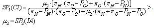 But if this is so, then it should also hold that:
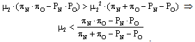 As we know from equation 1 that this last result is not true, then this is a contradiction. Therefore, “SP2(CI) < SP2(IA)”, q.e.d.With these results at hand, it is straightforward to prove that the average expected scoring probability is always higher under incomplete information, provided that “0 < θ < 1”. That is the theme of proposition 3.Proposition 3: If “0 < θ < 1”, then the average expected scoring probability is greater under incomplete information than under complete information.Proof: Recall that the expected scoring probabilities for the two types of kickers under the different analyzed cases are the following:
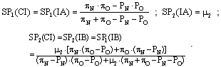 Let us now define the average expected scoring probabilities in the following way:
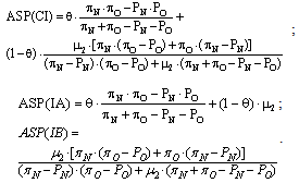 As we know (from lemma 2) that “SP2(IA) > SP2(CI)”, then we also know that “ASP(IA) > ASP(CI)”. And as we know (from lemma 1) that “SP2(CI) = SP1(IB) > SP1(CI)”, then we also know that “ASP(IB) > ASP(CI)”. Combining both results, it holds that, for any value of θ such that “0 < θ < 1”, it is true that “ASP(II) > ASP(CI)”, q.e.d.
4. Numerical Illustration
4.1. Theoretical Example
The results that we have obtained in section 2 can be illustrated for a particular set of parameters. Using the estimates that appear in[4], we will assume that “πN = 0.98”, “πO = 0.94”, “μ = 0.88”, “PN = 0.68” and “PO = 0.48”. This implies that, under complete information, the equilibrium values for n1, ν1, n2, c2, ν2 and γ2 are the following: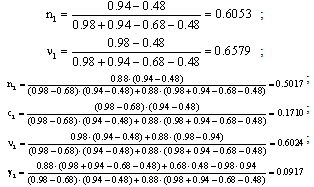 Given this, we can now calculate the expected scoring probabilities for these complete-information games, which are the following:
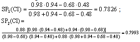 As we see, these results satisfy lemma 1, under which “SP2(CI) > SP1(CI)”.If we now turn to the incomplete-information situation, we have two possible cases depending on the fact that θ is either greater than or less than 0.82895. When “θ > 0.82895” (case A)4 ,it will hold that:
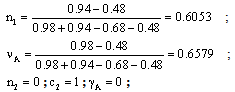 Where as, if “θ < 0.82895” (case B), it will hold that:
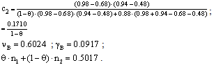 Besides, as we know from the results obtained in section 2, “SP1(IA) = SP1(CI) = 0.7826”, “SP1(IB) = SP2(IB) = SP2(CI) = 0.7993” and “SP2(IA) = μ2 = 0.88”. This implies that the average expected scoring probabilities under complete information and under the two incomplete-information cases are the following:
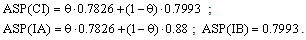 As we can see from the formulae, the incomplete-information cases produce some results that depend on the value of θ, that is, on the proportion of type 1 kickers that we have in the population under analysis. Figure 1 depicts the values of c2 and γM that we obtain as equilibrium values for all possible levels of θ, and in that figure we can see that c2 tends to its complete-information level when θ tends to zero, and becomes equal to one if “θ ≥ 0.82895”. The value of γM, correspondingly, jumps from a value equal to the strategy chosen for a complete-information situation where the goalkeeper faces kicker 2 (γM = 0.0917) to a value equal to zero, and this also occurs when “θ ≥ 0.82895”.
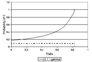 | Figure 1. Equilibrium strategies under incomplete information |
Correspondingly, figure 2 depicts the average scoring probability under complete and incomplete information for all possible levels of θ. In it we see that, unless “θ = 0” or “θ = 1”, the average scoring probability is higher under incomplete information. We also see that, when θ increases, the average scoring probability under complete information decreases (since “SP1(CI) < SP2(CI)”, and the average scoring probability is equal to “θ∙SP1(CI) + (1-θ)∙SP2(CI)”). The average scoring probability is also decreasing in θ under incomplete information if “θ > 0.82895”, but for the levels of θ that are below that threshold it is constant and equal to the maximum possible average scoring probability (i.e., “ASP(II) = 0.7993”).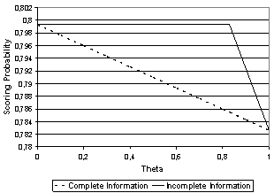 | Figure 2. Average scoring probabilities |
4.2. Empirical Application
The numerical examples that we have built in the previous section, although based on parameter values estimated using real data, are not a true empirical illustration of our incomplete-information models, since they just try to find out the equilibrium values for those models under certain assumptions. In this section we will get closer to an empirical application of the models using some data reported in four empirical studies about the penalty-kick game, and we will try to see if the use of an incomplete-information approach can be helpful to improve the results of an equilibrium estimation. The exercise, however, will fall short of an actual empirical estimation of an incomplete-information model, basically because we will not use the original data which are the source of the empirical studies, but only some descriptive statistics that we will take as estimates of the underlying strategies and parameters of the model. The aim of this illustration, therefore, will not be to test an incomplete-information model but simply to show a possible approach to the problem of estimation of such a model in four particular situations.The empirical studies that we will use as a source for our illustrations will be the already cited papers by Chiappori, Levitt and Groseclose[3], Palacios-Huerta[10], Bar-Eli et al.[1] and Baumann, Friehe and Wedow[2]. The first two of those studies give strong evidence in favor of thereasonableness of the complete-information Nash equilibrium as a solution for the penalty-kick game, while the third one questions that evidence. The study by Baumann, Friehe and Wedow, finally, does not test the complete-information model but presupposes its validity.| Table 2. Information from penalty-kick studies |
| | Concept | CLG | PH | BEA | BFW | | Average n | 0,4488 | 0,4980 | 0,3917 | 0,4374 | | Average c | 0,1721 | 0,0750 | 0,2867 | 0,1582 | | Average ν | 0,5665 | 0,5310 | 0,4441 | 0,5435 | | Average γ | 0,0240 | 0,0170 | 0,0629 | 0,0110 | | Implied πN | 0,9437 | 0,9648 | 1,0000 | 1,0000 | | Implied πO | 0,8992 | 0,9443 | 1,0000 | 1,0000 | | Implied μ | 0,8418 | 0,8820 | 0,9304 | 0,6537 | | Implied PN | 0,6320 | 0,7120 | 0,7460 | 0,4922 | | Implied PO | 0,4400 | 0,5520 | 0,7040 | 0,3569 | | Average Scoring Rate | 0,7490 | 0,8010 | 0,8530 | 0,7357 |
|
|
On table 2 we present a few data gathered from these four studies, which have been “translated” into our terminology of strategies (n, c, ν, γ) and scoring probabilities (πN, πO, μ, PN, PO)5. Of course, the numbers reported are not necessarily the actual strategies and probabilities but the average frequencies with which the players have chosen the different options (NS, OS and C) and the average scoring rates that occurred under the different combinations of those options. We also report the aggregate average scoring rates that correspond to the samples used in each of the studies. As the reader can imagine, “CLG” means Chiappori, Levitt and Groseclose, “PH” means Palacios-Huerta, “BEA” means Bar-Eli et al., and “BFW” means Baumann, Friehe and Wedow.Using the scoring rates that appear on table 2, it is relatively simple to calculate which would be the average Nash equilibrium strategies that players would have chosen if they had played in a complete-information environment. These are the ones predicted by equations 2, 3, 4 and 5, depending on the fulfillment of equation 1. To check this last condition it is necessary to calculate what we can call a “critical μ”, which is the maximum level of μ for which we can expect the occurrence of a restricted-randomization equilibrium. The first rows of table 3 show those complete-information equilibrium strategies implied by the four studies under analysis, together with the corresponding critical μ and the implied average scoring probability (ASP).| Table 3. Equilibrium results under complete and incomplete information |
| | Concept | CLG | PH | BEA | BFW | | Complete information | | | | | | Critical μ | 0,7400 | 0,8030 | 0,8633 | 0,7163 | | Implied n | 0,4881 | 0,5178 | 0,4692 | 0,5588 | | Implied c | 0,1807 | 0,1484 | 0,1281 | 0,0000 | | Implied ν | 0,5943 | 0,5936 | 0,5043 | 0,5588 | | Implied γ | 0,0991 | 0,0762 | 0,0629 | 0,0000 | | Implied ASP | 0,7584 | 0,8148 | 0,8719 | 0,7163 | | Incomplete information | | | | | | Estimated θ | 0,9367 | 0,9725 | 0,8347 | 0,8418 | | Implied n1 | 0,4791 | 0,5121 | 0,4692 | 0,5196 | | Implied n2 | 0,0000 | 0,0000 | 0,0000 | 0,0000 | | Implied c1 | 0,1162 | 0,0489 | 0,1455 | 0,0000 | | Implied c2 | 1,0000 | 1,0000 | 1,0000 | 1,0000 | | Implied ν | 0,6391 | 0,6296 | 0,5043 | 0,5588 | | Implied γ | 0,0240 | 0,0170 | 0,0629 | 0,0000 | | Implied ASP | 0,7578 | 0,8102 | 0,8719 | 0,7064 |
|
|
If we now compare the complete-information equilibrium results from table 3 with the information reported on table 2, we can see some striking similarities but also some important differences, which may cast some doubts about the ability of the complete-information model to explain the players’ behavior. The implied average scoring probabilities, for example, are very similar to the actual average scoring rates in the four cases. The implied values of c for the CLG study, of n for the PH study, and of γ for the BEA and BFW studies are also extremely similar to the average values reported on table 3. Conversely, we can see that the calculated complete-information equilibrium predicts implied values for the parameters that are very different to the reported average values for the cases of the parameters n and c in both the BEA and BFW studies, for the parameters c, ν and γ in the PH study, and also for the parameter γ in the CLG study. Moreover, the complete-information model predicts that the equilibrium in the BFW study should be one of restricted randomization (since the critical μ is larger than the parameter μ implied by the data), but we nevertheless observe a relatively large fraction of kicks that were actually shot to the center of the goal by the kickers in that sample.Some of these divergences can be partially explained using a few easy incomplete-information assumptions like the ones made to calculate a new set of implied parameters (which are the ones that appear in the last rows of table 3). For the CLG case, for example, we have assumed two types of kickers: type-2 kickers strictly prefer to shoot to the center of the goal, while type-1 kickers choose a mixed strategy that combines NS, OS and C with positive probability. To match the data on the observed choices of NS, we had to assume a certain distribution of the types (the “estimated θ”), and based on that we also estimated a certain value for the implied parameter c1. The parameter γ, conversely, was supposed to be equal to the observed average value for that parameter, while ν was estimated as the value that made type-1 kickers indifferent between choosing NS, OS and C.The same methodology for defining the two types of kickers were used to match the data reported in the PH and BEA studies. For the BFW study, however, we had to use a different approach to conciliate the prediction of the complete-information model (that on average it was not optimal for the kickers to choose C) with the data that show that 15.82% of the kicks were actually shot to the center of the goal6. In order to solve that puzzle, we assumed that in this case type-1 kickers were players who never chose C and type-2 kickers were players who always shot to the center of the goal. These assumptions allowed us to estimate a certain value for θ, but obliged us to assume that the implied value for γ was equal to zero. This last feature does not exactly match the data (since the average γ in the BFW study is 0.011), but it helps us to explain how it is possible that there is such a large fraction of kickers that choose C in equilibrium while almost no goalkeeper is willing to stay in the center of the goal.
5. Conclusions
The main conclusions of this paper have to do with the idea that, in some cases, the outcomes of a situation in which a soccer goalkeeper faces a kicker at a penalty kick can be better explained as the result of an incomplete-information game. In those cases, the relevant solution concept is no longer the mixed-strategy Nash equilibrium of the game but the corresponding Bayesian equilibrium, since at least one of the players (e.g., the goalkeeper) is facing uncertainty about his opponent’s type.In the simplified model that we presented, we see that, under incomplete information, the typical situation is that one of the kicker’s types is responding to a strategy that the goalkeeper has designed for a different type of opponent. Being unable to distinguish among the different types, the goalkeeper has to play the same strategy against every opponent, and this is why some types of kickers may prefer a pure strategy. When we mix the strategies played by the different kickers, however, we end up with a sort of “average kicker strategy” with different probabilities for the available pure strategies, and this average strategy has to be such that the goalkeeper is indifferent between playing the pure strategies that he mixes when he chooses his own best response to the “expected kicker”.We have also found cases in which one of the kicker’s types plays a “restricted mixed strategy” (e.g., one that randomizes between NS and OS) while the other type plays a “full mixed strategy” (i.e., one that randomizes among NS, OS and C). Moreover, we can also end up in a situation in which one of the kicker’s types plays a restricted mixed strategy and the other one plays a pure strategy, and the goalkeeper chooses a restricted mixed strategy himself (which is the best response to the kicker who plays the restricted mixed strategy). This last case produces the apparently paradoxical situation that, in equilibrium, the goalkeeper never chooses the center of the goal while one of the kicker’s types always shoots to that place.The relative lack of information that the goalkeeper faces in a situation of incomplete information makes the average scoring probability higher than under a situation of complete information, which is equivalent to say that, on average, the kicker is better off under incomplete information and the goalkeeper is worse off. This feature can therefore be used to find the “value of information” in this game. As goalkeepers’ payoffs are the complements of the scoring probabilities, the value of knowing the true characteristics of a kicker can be measured as the difference between the expected scoring probability under complete and incomplete information. This difference is smaller if we are in a situation in which uncertainty is small (i.e., when the parameter θ, which measures the distribution of the kicker’s types, is very close to zero or to one) and becomes larger when we approach the level of θ where the Bayesian equilibrium of the game changes from case A to case B. The difference will also be larger if the different types of kickers are “more different” among themselves.Another virtue that the incomplete-information approach could have is to solve some puzzles that the empirical literature on penalty kicks has discovered. Indeed, we have seen on section 4 that the Nash equilibrium concept performs quite well to explain some phenomena observed in a number of empirical studies about penalty kicks, but that some other features are hard to explain using a complete-information approach. This is particularly true for the relatively widespread fact that concerns shots to the center of the goal, which are typically more common than what a complete-information Nash equilibrium predicts. This feature of the complete-information model has been criticized by Bar-Eli et al.[1] as a weakness of the game-theoretic approach, and it has been explained by those authors using norm theory.By introducing incomplete information, however, the situation described in the previous paragraph can be explained as the result of a game-theoretic equilibrium. Without recurring to psychological arguments, we have seen that it can be optimal for a goalkeeper to randomize between NS and OS although he knows that a group of kickers will always choose C, provided that such a group of kickers is relatively small. We have also seen that it is possible to think of certain Bayesian equilibrium solutions in which the goalkeeper randomizes among NS, OS and C, and the different types of kickers choose more restricted mixes (e.g., between NS and OS) or even pure strategies.The main analytical problem of introducing incomplete information into the penalty-kick game may perhaps be its extreme capacity to match the data. Indeed, if we build a game of incomplete information that postulates more than two types of players and we arbitrarily use different probabilities for those types, then we could probably explain any dataset on penalty kicks as a result of a particular Bayesian equilibrium. If that is the case, then many of the empirical tests that the game-theoretic penalty-kick literature has designed could become useless, since it would actually be impossible to distinguish between a Bayesian equilibrium and a situation in which the players are not choosing their strategies rationally.We nevertheless believe that the Bayesian equilibrium concept also opens the door for new possible empirical estimations of the penalty-kick game, especially in cases in which it is not clear whether the goalkeepers know their opponents’ types. This is particularly true for situations in which the expected incomplete-information solution is markedly different from the expected complete-information solution, and especially when we can somehow divide a sample of penalty kicks into different types of kickers7. In those cases, it could be possible to contrast the predictions of the complete-information Nash equilibrium concept with the ones of the incomplete-information Bayesian equilibrium concept, and also with other alternative concepts that are foreign to the game-theoretic approach.
ACKNOWLEDGEMENTS
I thank Nicolás Caputo, Pierre-André Chiappori, Timothy Groseclose, Hugo Hopenhayn, John Riley, Connan Snider, Jorge Streb and one anonymous referee, for their useful comments. I also thank the participants of two seminars held at CEMA University and at the University of California, Los Angeles.
Notes
1. In fact, this model is basically the same that was originally presented by Chiappori, Levitt and Groseclose[3].2. This last feature has to do with the fact that, in our model, both kickers have the same values for “πN”, “πO”, “PN” and “PO”. If there were some differences in these values for the two types of kickers, then kicker 1 might strictly prefer either NS or OS.3. In the working-paper version of this article (Coloma[5]) we have included a detailed description of these restrictions. That working-paper version also includes a simplified two-strategy version of the penalty-kick model.4. This number comes from substituting the values of πN, πO, PN, PO and μ2 into the formula found in propositions 1 and 2, which are the ones that define the range of values of θ for which case A and case B equilibria can occur. 5. In three of the four cases the calculations were relatively easy, because the studies reported either the actual frequencies and rates or the actual number of shots needed to calculate those rates. For the case of[2], conversely, we had to apply a very indirect method to detect the implied scoring rates in each of the strategy profiles. 6. Of course, this implies assuming that type-2 kickers are players whose scoring probabilities when shooting NS or OS are completely different (lower) than the ones associated to type-1 kickers. These lower scoring probabilities are never observed, since type-2 kickers always choose C instead of NS or OS.7. This division may rely on phenomena that are not ex-ante observed by goalkeepers but are ex-post observed by the analyst (e.g., if a kicker never chooses a certain action, the speed of the shots that he kicks, etc.).
References
| [1] | Bar-Eli, Michael; Azar, Ofer; Ritov, Ilana; Keidar-Levin, Yael and Schein, Galit (2007). “Action Bias Among Elite Soccer Goalkeepers: The Case of Penalty Kicks”; Journal of Economic Psychology, vol 28, pp 606-621. |
| [2] | Baumann, Florian; Friehe, Tim and Wedow, Michael (2011). “General Ability and Specialization: Evidence from Penalty Kicks in Soccer”; Journal of Sports Economics, vol 12, pp 81-105. |
| [3] | Chiappori, Pierre-André; Levitt, Steven and Groseclose, Timothy (2002). “Testing Mixed-Strategy Equilibria when Players are Heterogeneous: The Case of Penalty Kicks in Soccer”; American Economic Review, vol 92, pp 1138-1151. |
| [4] | Coloma, Germán (2007). “Penalty Kicks in Soccer: An Alternative Methodology for Testing Mixed-Strategy Equilibria”; Journal of Sports Economics, vol 8, pp 530-545. |
| [5] | Coloma, Germán (2012). “The Penalty-Kick Game under Incomplete Information”, Working Paper No. 487. Buenos Aires, CEMA University. |
| [6] | Dohmen, Thomas (2008). “Do Professionals Choke under Pressure?”; Journal of Economic Behavior and Organization, vol 65, pp 636-653. |
| [7] | Harsanyi, John (1967). “Games with Incomplete Information Played by Bayesian Players”; Management Science, vol 14, pp 159-182. |
| [8] | Jabbour, Ravel and Minquet, Jean (2009). “Goalkeeper Strategic Valuation”, mimeo; Ecole Supérieure des Affaires, Beirut. |
| [9] | Moschini, Gian Carlo (2004). “Nash Equilibrium in Strictly Competitive Games: Live Play in Soccer”; Economics Letters, vol 85, pp 365-371. |
| [10] | Palacios-Huerta, Ignacio (2003). “Professionals Play Minimax”; Review of Economic Studies; vol 70, pp 395-415. |
| [11] | Pollard, Richard; Ensum, Jake and Taylor, Samuel (2004). “Estimating the Probability of a Shot Resulting in a Goal: The Effects of Distance, Angle and Space”; International Journal of Soccer and Science, vol 2, pp 50-55. |
| [12] | Savage, David and Torgler, Benno (2009). “Nerves of Steel?: Stress, Work Performance and Elite Athletes”, Working Paper No. 251. Brisbane, Queensland University of Technology. |
 Abstract
 Reference
 Full-Text PDF
 Full-Text HTML