Masamichi Kawano1, Kazuhiro Ohnishi2
1School of Economics, Kwansei Gakuin University, Japan
2Institute for Basic Economic Science, Japan
Correspondence to: Kazuhiro Ohnishi, Institute for Basic Economic Science, Japan.
| Email: |  |
Copyright © 2012 Scientific & Academic Publishing. All Rights Reserved.
Abstract
Interesting explanation of an adjustment process in a Cournot duopoly game is shown in Varian[1]’s textbook, where players adjust their strategies sequentially. It is generally assumed that players adjust simultaneously. We investigate a game that determines whether to adjust or not. First, Nash principle is assumed and as the solution whether sequential or simultaneous is derived. The result depends on the initial state of the output of both firms. In some regions firms adjust simultaneously, and in other regions sequentially. The game under maximin principle is also examined and we compare the results with that of the Nash game.
Keywords:
Adjustment Process, Cournot Duopoly, Nash Game, Maximin Game
1. Introduction
The assumption of Cournot[2] model has been the most widely used in analyzing quantity-setting oligopoly games. Varian[1] explains a process of adjustment to Cournot equilibrium as follows. He considers a Cournot game in which there are two firms (firm 1 and firm 2). Suppose that in period 1 the firms are producing outputs , where superscripts denote time periods and subscripts denote firms. If firm 1 expects that firm 2 is going to continue to keep its output at
 , then in period 2 firm 1 would want to choose its profit maximizing output given
 . Hence, firm 1’s choice in period 2 will be given by
 , where
  denotes firm 1’s reaction function. Firm 2 can reason the same way, and therefore firm 2’s choice in period 2 will be
 , where
  is firm 2’s reaction function. These equations describe how each firm adjusts its output in the face of the rival’s choice. These behaviors of the firms are illustrated in Figure 1, where the horizontal axis denotes firm 1’s output, the vertical axis is firm 2’s output,
  is firm 1’s reaction curve, and
  is firm 2’s reaction curve.We start with some initial point
 . Given
 , firm 1 optimally chooses to produce
  in period 2. Hence, the state moves horizontally to the left until
  on
on . If firm 2 expects firm 1 to continue to produce
 , then its optimal response is to produce
 . Therefore, the state moves vertically upward until
  on
on . Furthermore, if firm 1 expects firm 2 to continue to produce
 , then the best firm 1 can do is to produce
 . Therefore, the state moves horizontally to the left until on
 . Hence, the state continues to move along the “staircase” to determine the sequence of output choice of two firms. In the end, the state reaches point
 .1 In this adjustment process, each firm assumes that the rival’s output will not change from one period to the next. Therefore, each firm keeps changing its output sequentially.2 This adjustment process converges to the Cournot equilibrium.
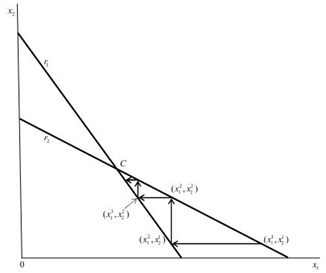 | Figure 1. Adjustment process to equilibrium under sequential adjustment |
We investigate a Cournot duopoly model that endogenously determines the process of adjustment to equilibrium. To the best of our knowledge, there is no previous work dealing with such situation. First, we assume that a Nash game is played at the initial operating point. It is then shown that there exist two possible cases as the result of the game: (1) both firms adjust their outputs simultaneously, and (2) only one firm adjusts its output after the rival’s adjustment and sequentially moves to the Cournot equilibrium. Next, we assume that a maximin game is played. It is then shown that there exists a difference in adjustment process compared with Nash game. As the result of these analyses, we find that there are cases in which Varian’s adjustment process illustrated in Figure 1 is not achieved.The remainder of this paper is organized as follows. In Section 2, we describe the model and investigate the Nash equilibrium to determine the adjustment process of the model. Section 3 examines the maximin principle to play the game to derive the adjustment process of the model. Finally, Section 4 concludes the paper.
2. Model and Nash Adjustment Process
Let us consider a market in which there are two firms. The firms face a downward-sloping inverse demand function . The subscripts 1 and 2 denote firm 1 and firm 2, respectively. In the remainder of this paper, when i and j are used to refer to firms, they should be understood to refer to 1 and 2 with
 . There is no possibility of entry or exit.Firm i’s profit function is given by
 , where
  denotes the constant marginal cost. We normalize the marginal cost to zero for the sake of simplicity.The formal definition of Nash equilibrium is as follows. A set of strategies is a Nash equilibrium if no firm has incentive to deviate from its strategy given the other firm plays its Nash equilibrium strategy.
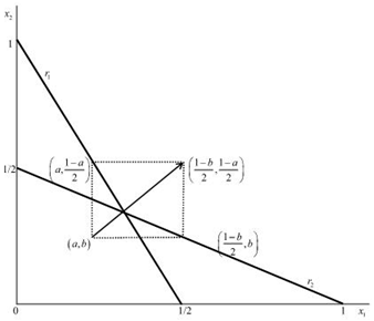 | Figure 2. Adjustment process from initial output levels  under simultaneous adjustment under simultaneous adjustment |
We now consider Figure 2, where (a, b) is initial output levels. If firm 1 adjusts its output and firm 2 does not, then the state will reach , while if firm 2 adjusts its output and firm 1 does not, then the state reaches
 . Furthermore, if both firms adjust their outputs, then the state will reach
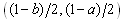 . Hence, the strategies for each firm are “adjust (A)” and “don’t adjust (D)”.This market is an example of a 2-by-2 game, because each of the two firms has two possible actions in its action set. The solution of the game is obtained by the output adjustment of firms. Therefore, the matrix of this game is as follows.
 At
At , a firm necessarily adjusts its output when the other firm does not, provided that the former is not on its reaction curve, since
 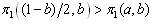 and
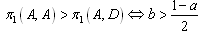
and 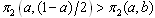 necessarily hold. This is made clear by the definition of the reaction function. Firm i’s optimal strategy is to choose A if firm j choose D. On the other hand, if firm i chooses A, then firm j’s choice is not determined. If
  is satisfied, then firm 1 will choose D, and the condition for this is
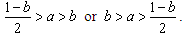 | (1) |
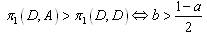
Similarly, if is satisfied, then firm 1 chooses D, and the condition for this is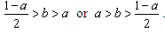 | (2) |
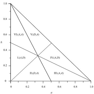 | Figure 3. Six regions in quantity space |
We divide the quantity space into six regions as depicted in Figure 3. We should note that since the price, which is given by , should be nonnegative, we have
 .The profits of regions (I-VI) in Figure 3 are as follows:I.
  ,II.
,II.  ,III.
,III.  ,IV.
,IV.  ,V.
,V.  ,VI.
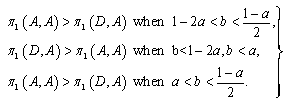
,VI.  ,where, for instance,
  implies the profit of firm i when the equilibrium strategy is (A,D). We can derive the Nash equilibrium considering the relative magnitude of the profits of firm 1 and 2 shown in the above. Thus we obtain the following proposition.Proposition 1. In the regions in Figure 3, the Nash equilibria are as follows: I (A, D), II (D, A), III (A, A), IV (A, D), V (D, A), and VI (A, A).
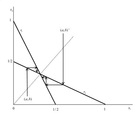
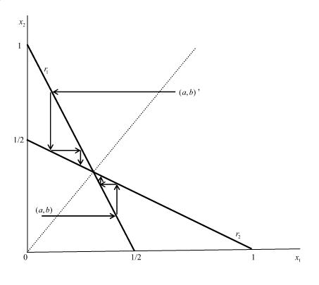 | Figure 4. Adjustment process when the equilibrium is at (A, D) |
 | Figure 5. Adjustment process when the equilibrium is at (D, A) |
In (A, D), the state moves horizontally to the right until a point on . In (D, A), the state moves vertically until a point on
 . After that, the two firms sequentially determine their output levels. Figures 4, 5 and 6 illustrate the movement of the outputs of the firms implied by this adjustment process. As was mentioned before, Varian’s adjustment process is achieved if the initial point is in the regions except III and VI in Figure 3. On the other hand, in III and VI, since the Nash equilibrium is (A, A), Varian’s adjustment process is not achieved because both firms adjust their outputs simultaneously.
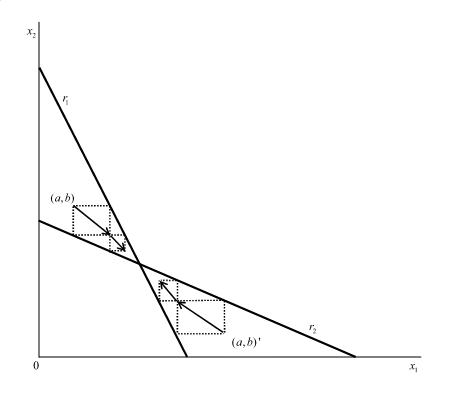 | Figure 6. Adjustment process when the equilibrium is at (A, A) |
3. Maximin Adjustment Process
In this section, we consider the maximin principle3. The optimal strategy of maximin principle is given by . At first, firm 1 searches the rival’s strategy which minimizes firm 1’s pay-off. Next, firm 1 finds the best strategy of its own to maximize its own pay-off. In this game, when
 | (3) |
 | (4) |
 | (5) |
 | (6) |
Similarly, the optimal strategies of firm 2 can be derived. Thus we obtain the following proposition.Proposition 2. In the regions in Figure 7, the Nash equilibria are as follows: I (A, D), II (D, A), III (A, A), IV (A, A), V (A, A), and VI (A, A).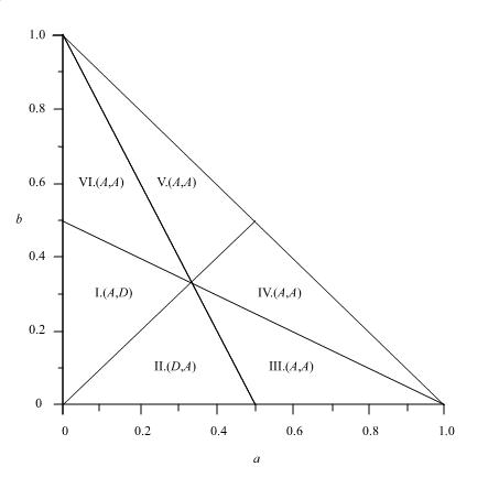 | Figure 7. Optimal strategies of the firms |
In Figure 7, we show the equilibrium strategies of the two firms. Comparing this figure with Figure 3, minor difference exists. That is, in the regions IV and V, the equilibrium strategy under maximin principle is (A,A), while under Nash strategy is (A,D) and (D,A), respectively. The optimal adjustment process under maximin principle starting from region V is shown in Figure 8. As shown in the figure, the first step jumps to region I, however, the second step hits the reaction curve of firm 1, ( ), then afterwards, the process is sequential.
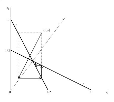 | Figure 8. Adjustment process when the equilibrium is at (A, A) |
4. Conclusions
We have investigated a Cournot duopoly model that endogenously determines the process of adjustment to equilibrium. First, we have assumed that a Nash game is played. We have demonstrated that there are two possible cases: (1) Varian’s adjustment process is achieved because only one firm adjusts its output at each period, i.e., the firms adjust sequentially one after another. (2) Varian’s adjustment process is not achieved because both firms adjust their outputs simultaneously. Next, we have assumed that a maximin game is played. We have shown that a difference exists between those two games. In the region of the output space where both firms have to reduce their outputs, i.e., the point outside of the reaction curves, the equilibrium of maximin game is (A,A), that is, both firms adjust simultaneously. Hence, at the next period, the state of the outputs comes into inside of the reaction curves. Then, there the equilibrium strategy is (A,D) or (D,A), and the sequential adjustment process starts. On the other hand, in Nash game, if the game started from that point, the Nash equilibrium is (A,D) or (D,A), then the sequential adjustment begins from the first period.
Notes
1. Also Varian[3] explains similarly, however, the graphical explanation is somewhat different, and it seems simultaneous adjustment process. The first and the second version of this book gave a definitely sequential graphical explanation.2. Okuguchi and Szidarovszky[4] examined the stability property of sequential adjustment process in multiproduct oligopoly game.3. For texts, see, e.g., [5-7]. See also [8].
References
| [1] | Varian, H. R., Microeconomic Analysis, 3rd ed., W. W. Norton & Company, USA, 1992. |
| [2] | Cournot, A. A., Récherches sur les Principles Mathématiques de la Theorie des Richesses. Hachette, France, 1838. English edition (Bacon, N. T., Researches into the Mathematical Principles of the Theory of Wealth. Macmillan, UK, 1897.) |
| [3] | Varian, H. R., Intermediate Microeconomics: A Modern Approach, 8th ed., W. W. Norton & Company, USA, 2010. |
| [4] | Okuguchi, K., Szidarovszky, F., The theory of Oligopoly with Multi-Product Firms, 2nd ed., (Lecture Notes in Economic and Mathematical Systems), Springer-Verlag, Germany, 1999. |
| [5] | Montet, C., Serra, D., Game Theory and Economics, Palgrave Macmillan, USA, 2003. |
| [6] | Vega-Redondo, F., Economics and the Theory of Games, UK, 2003. |
| [7] | Rasmusen, E., Games and Information: An Introduction to Game Theory, 4th ed., Blackwell Publishing, USA, 2007. |
| [8] | Grafton, R. Q., Nelson, H. W., Lambie, N. R., Wyrwoll, P. R., A Dictionary of Climate Change and the Environment: Economics, Science, and Policy, Edward Elgar Publishing, UK, 2012. |
 Abstract
 Reference
 Full-Text PDF
 Full-Text HTML