Zhifan Han, Xin Wang, Dong Zhao
School of Civil and Transportation Engineering, Guangdong University of Technology, Guangzhou, China
Correspondence to: Zhifan Han, School of Civil and Transportation Engineering, Guangdong University of Technology, Guangzhou, China.
| Email: |  |
Copyright © 2017 Scientific & Academic Publishing. All Rights Reserved.
This work is licensed under the Creative Commons Attribution International License (CC BY).
http://creativecommons.org/licenses/by/4.0/

Abstract
Numerical simulation on wind pressure of high-rise buildings needs to set up a corresponding numerical wind tunnel model for different wind directions. The cylindrical computational domain in numerical modeling realizes the sharing of numerical models for different wind directions. It significantly reduces the repeated modeling construction work and improves the efficiency of numerical simulation. Based on the wind tunnel test of atmospheric boundary layer, this paper compares the experimental results of numerical wind tunnel simulation of wind pressure on high-rise buildings with those from TJ-2 (Tongji University Wind-tunnel Laboratory) and NPL (National Physical Laboratory). Cylindrical computational domain is verified to be feasible and no extra numerical errors were introduced when used in the simulation process. Throughout the analysis of different cylindrical computational domain sizes, an appropriate size of cylindrical computational domain is proposed, which provides references for both CWE (Computational Wind Engineering) and researches on atmospheric boundary simulation.
Keywords:
Numerical simulation, Computational wind engineering, Cylindrical computational domain, Open boundary
Cite this paper: Zhifan Han, Xin Wang, Dong Zhao, Wind Pressure on High-rise Buildings: A Numerical Simulation of Computational Domain, Journal of Civil Engineering Research, Vol. 7 No. 2, 2017, pp. 46-52. doi: 10.5923/j.jce.20170702.02.
1. Introduction
In the numerical simulation of structural wind engineering, cases of different wind directions need to be calculated, and corresponding numerical wind tunnel models should be set up. This means repeated work of computational domain construction, grid discretization and boundary condition definition, which causes extra work and is time-consuming. Besides, the computational domain size directly influences the authenticity and workload of the simulation results. If the simulation domain is small, the flow field will be distorted; whereas, if excessively enlarged, the calculation work and cost will increase. An appropriate selection of computational domain will guarantee the accuracy of the simulation results without increasing the amount of calculation. Among the current researches on wind engineering numerical simulation, many researchers have already attached much attention to the selection of computational domain. Xinyu Wen conducted CFD simulation of outdoor wind environment in residential planning and construction by selecting a rectangular area along the coming flow direction. To satisfy the calculation accuracy, he set the following dimensions based on experience--- the height and the width of computational domain are 3 and 6 times those of the building, the distances between the building and the inflow and outflow boundaries are 3 and 4 times the width of the building respectively [1]. Yang jie, etc. conducted wind environment simulation of a high-rise residential building. He set the height of the computational domain 3 times that of the building, the distances between the building and inflow and outflow boundaries and the width of the domain is 3, 10 and 6 times the width of the building [2]. European Cooperation in the Field of Scientific and Technical Research (COST) specifies that the size of computational domain in height, horizontal, and the flow direction depends on the area described and the boundary conditions (for single buildings the top of the computational domain should be set at least 5H above the roof of the building, where H is the height of the single building or the tallest building in buildings) [3]. AIJ wind engineering research team expresses that the blockage ratio should be below 3% based on the wind tunnel experiments. For the single-building, the lateral and the top boundary should be set 5H or more away from the building, where H is the height of the target building. The distance between the inlet boundary and the building should be set in consistency with the upwind area of the wind tunnel. The outflow boundary should be set at least 10H behind the building [4, 5]. Based on the wind tunnel test of atmospheric boundary layer, the numerical wind tunnel simulation results of high-rise building are compared with those of TJ-2 and NPL [6], the geometry model of the computational domain is proposed to be designed into cylinder with calculation model in the center rotating around its axis. For the different wind directions, the computational domain could remain unchanged by just spinning the axis to the needed angle. This realizes the sharing of numerical models for different wind directions. In this way, the efficiency of numerical modeling simulation in wind engineering is highly improved and the numerical simulation period is shortened. To find out the appropriate size of computational domain, a variety of computational domain cases for numerical simulation analysis were designed so that the computational domain would not be too large and the error between calculated results and the actual value would not be affected.
2. Numerical Simulation
2.1. The Basic Control Equation of Fluid Flow
Buildings lie in all kinds of gradient wind field at low speed, so the incompressible viscous fluid model is adopted. In the neutral atmospheric stratification without temperature changes in the flow field, the governing equations of the incompressible turbulent wind flow around buildings are presented by the RANS equations as follows:(1) mass conservation equation: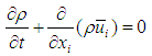 | (1) |
(2) momentum conservation equation: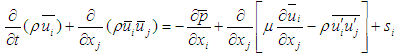 | (2) |
Where ρ is the fluid density, µ is the dynamic viscosity,  is the Reynolds stress,
  is the source term, equation (2) from left to right in turn called transient item, convection item, diffusion item and the source term. With the term of Reynolds stress included in the above equation, equation is not closed, so it is necessary to find the corresponding appropriate turbulence model [7].
2.2. Turbulence Model
The Shear Stress Transport (SST) k-ω turbulence model proposed by Menter is highly precise when simulating turbulent flow, for it considers turbulent shear stress transport in the adverse pressure-gradient boundary layer. The numerical simulation of the flow around the standard building model indicates that it is suitable to be applied in the numerical simulation of bluff body flow [8, 9]. Wilcox k-ω model is applied in the near wall regions of k-ω model, and k-ε model is applied in the free shear layer, during which a blending function is used, whose governing equation is given as following: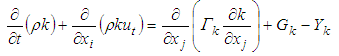 | (3) |
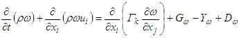 | (4) |
Where  is the generation of ω;
  and
and  are the convective terms of k and ω, respectively;
  and
and  are the dissipation terms of generation of k and ω, differently [10, 11].SST k-ω model add the cross diffusion term
  compared with the standard k-ω model in equation, and the spread of the turbulent shear stress is considered in turbulent viscosity which enables SST k-ω model to have higher accuracy than the standard k-ω model in flow field.
3. Numerical Model Validation
3.1. Calculation Model
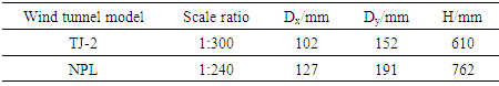
The size of experimental model is shown in Table 1. Dx and Dy are cross section width and cross section length of model, respectively, H as the height of model. It prescribes that 20 pressure taps are set as standard pressure tap locations at 2/3 model height. The model and surface pressure tap locations are shown in Figure 1.Table 1. Model Size
 |
| |
|
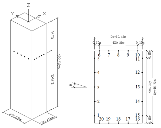 | Figure 1. CAARC standard model and layout of pressure taps at 2/3 model height |
3.2. Computational Simulation Setting
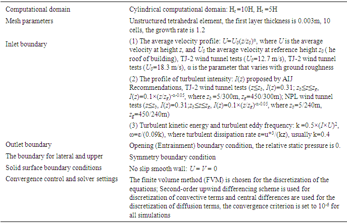
The computational domain uses the cylindrical computational domain, with the building model in the center. And radius of cylindrical computational domain (Hr) is 10H, the top of the computational domain above the roof of the building (Ht) is set 5H, where H is the height of the building (Figure 2). The computational domain should not exceed the recommended blockage ratio (3%) [4]. The settings of boundary conditions and simulation control parameters are shown in Table 2.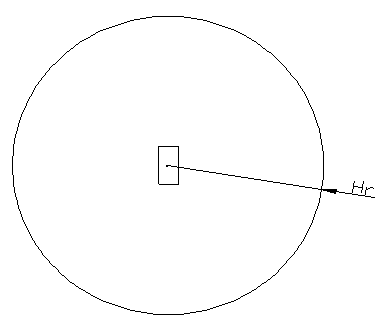 | Figure 2. The size of fluid computational domain |
Table 2. The Settings of the Boundary Condition and Control Parameters
 |
| |
|
3.3. Analysis of Results
Use the ANSYS-CFX software to simulate the computational fluid dynamics (CFD) model of building at the wind angle of 0°. The comparisons of experimental measurements (TJ-2 wind tunnel tests and NPL wind tunnel tests) with the mean pressure coefficients at 2/3 model height (pressure taps as shown in Figure 1) are shown in Figure 3 and 4, respectively. The mean wind pressure coefficients are represented as: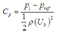 | (5) |
Where  is the mean local pressure due to the wind at a point i(Pa),
  is static pressure far from the building influence zone (1.01325×10⁵Pa), ρ=1.225 kg/m3 the air density and Ub the reference wind speed at the top of building.
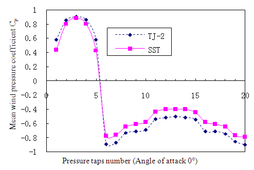 | Figure 3. Comparison of CP by CFD simulation results of B types of roughness and TJ-2 wind tunnel experiments |
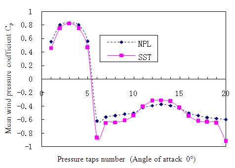 | Figure 4. Comparison of CP by CFD simulation results of D types of roughness and NPL wind tunnel experiments |
From Figure 3 and 4, it could be concluded as follows:1) At the windward facade, the numerical simulation results share the same trend with those from the wind tunnel tests, and the pressure coefficients of the pressure taps are similar.2) At the leeward facade, overall, simulation results are more close to the NPL experimental results. For B types of roughness, the CFD results share the same trend with TJ-2 experimental results, but individual point deviation is relatively apparent. While for D types of roughness, the trend in the numerical predictions for the Cp is in a good agreement with the experimental results.3) On side face, the simulation results have certain deviation with the test results due to separation of the flow, but a good agreement can be observed in the change curve. The simulation results of tap 6, 7, 19, 20 in terrain category-D deviate largely from the NPL test data, the same with the terrain category-B, because the angle is not guaranteed 90° in the model making of wind tunnel test. However, their change curve, showing values with good approximation, meets the engineering requirements.Overall, the CFD and wind tunnel results have good consistency in terms of wind pressure distribution and wind pressure changing tendency, which proves the precision and reliability of cylindrical computational domain.
4. Numerical Simulation of the Computational Domain
4.1. Simulation Design
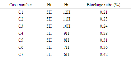
Employ CAARC standard model for high-rise building, and the dimension of building model is 152mm(L)×102mm(B)×610mm(H). The geometrical scale was 1/300 for the CAARC scale model. The real dimension for the CAARC standard model of high-rise building was about 45.72m(L)×30.48m(B)× and 182.88m(H). The average wind velocity has been maintained as 12.7 m/s at the roof level of the model. Reynolds number (Re) based on the model height is 4.9×10⁶, which is greater than the ASCE recommended Reynolds number 11000 [12]. Thereby, it can be inferred that simulation results are independent of wind velocity.In the present paper, in order to examine the effects of cylindrical computational domain size on the numerical simulation results, seven configurations of the cylindrical computational domain have been designed. Assume the height of cylindrical domain Ht =5h and its radius Hr=6H, 7H, 8H, 9H, 10H, 11H, 12H (H is the height of the target building), which represents seven different sizes of cylindrical domains. In principle, the blockage ratio should not exceed 3%. Through the numerical simulation of the seven computational domains in different sizes, the outlet velocity u, turbulence kinetic energy k and turbulent dissipation rate ε have been obtained, satisfying the zero pressure gradient variables accordingly. Through the analysis and comparison, the optimal computational domain was obtained as small as possible without influencing the precision of numerical results. Calculation model is shown in Figure 5 and project design is shown in Table 3, respectively.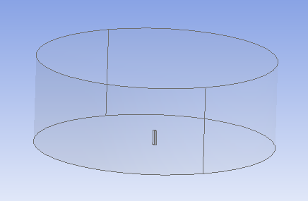 | Figure 5. Isometric views of the computational model |
Table 3. Design of Simulation Cases of the Fluid Computational Domain
 |
| |
|
4.2. Computational Simulation Settings
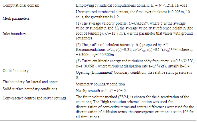
The settings of boundary conditions and simulation control parameters are shown in Table 4.Table 4. The Settings of the Boundary Condition and Control Parameters
 |
| |
|
5. Results and Discussion
Select a horizontal line at height level 0.5m, and analyze the change law of outlet velocity u, turbulent kinetic energy k and turbulence dissipation rate ε with the distance away from the leeward side of building. The change trend curve of u, k, ε with the increase of Hr is plotted in Figure 6(a), 6(b) and 6(c), respectively.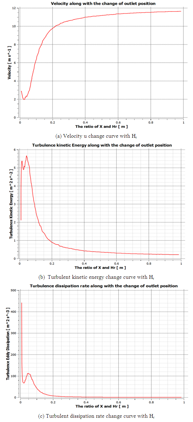 | Figure 6. The value of u, k, ε change curve with Hr |
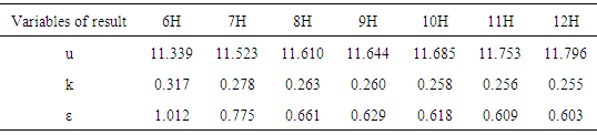
As can be seen from Figure 6, the values of velocity u, k, ε generate a great change of gradient and produce mutations in the leeward side of building, because the outlet boundary close to the building wall lies in the wake zone with backflow. Provided that such outlet is configured, the assumed zero gradient will not meet the conditions, and a reverse flow zone will be generated. Therefore, flow may not be able to reach the state of full development, which will greatly influence the accuracy of the calculation results. Furthermore, with the increase of interval between outlet and the leeward side of building, the values of u, k, ε begin to flatten slowly until its changing gradient approximates 0, then each variable meets the zero gradient boundary condition at the outlet, so as to obtain more accurate results. Therefore, it can be concluded that a good agreement is acquired between the numerical result and actual value with the length of the leeward facade increasing.For further analysis, Hr was increased gradually for numerical simulation. Under each condition the values of u, k, ε at 0.5m height outlet (angle of attack 0o) are presented in Table 5. Values of u, k, ε are plotted in Figure 7, 8 and 9, and analysis is made to the numerical results.Table 5. The Value of u, k, ε under the Condition of the Different Computational Domain
 |
| |
|
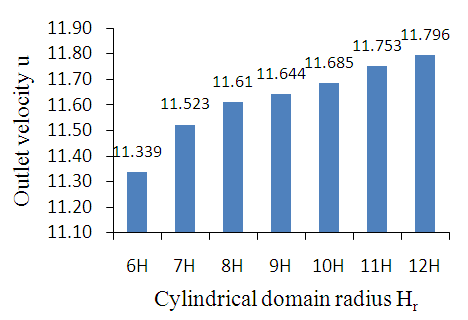 | Figure 7. Outlet velocity change curve with Hr |
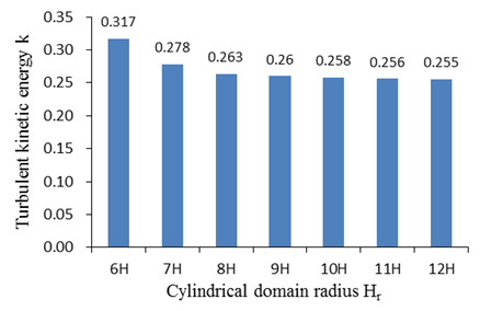 | Figure 8. Turbulent kinetic energy change curve with Hr |
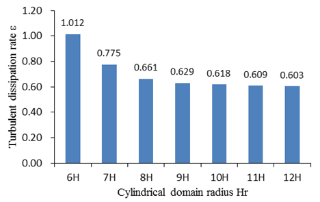 | Figure 9. Turbulent dissipation rate change curve with Hr |
Each condition represents a different computational domain size, and the radius of computational domain increases gradually. From Figure 7, 8 and 9, it can be inferred: (1) For the outlet velocity u, with the increase of computational domain radius Hr at outlet location, it increases gradually and tends to level off until it approximates the real wind velocity at 0.5m high (u0.5=12.3m/s). The relative error for Hr between 6H and 7H is approximately 1.62% and it is 0.37% ~ 0.76% for each condition after Hr exceeds 7H. It could be inferred that the size of computational domain would not influence the outlet velocity u as long as Hr is at least 7H.(2) For turbulent kinetic energy k, it decreases with the increase of Hr and flattens after Hr exceeds 7H. The relative error for Hr between 6H and 7H is 12.3%, between 7H and 8H is 5.39% and after 8 H, the relative error for other conditions is 0.39%~1.14%. Therefore, it could be inferred that the size of computational domain would not influence the turbulent kinetic energy k as long as Hr is at least 8H.(3) For turbulent dissipation rate ε, it decreases with the increase of Hr and flattens after Hr exceeds 7H. The relative error for Hr between 8H and 9H is 4.84%, and it decreases with the Hr increasing. Above all, if cylindrical computational domain is employed, then it is suggested that Hr is not less than 8H. Also, the oversize of numerical wind tunnel will enlarge the calculation workload, so 8H~10H is more appropriate and preferable when selecting the size of the cylindrical computational domain.
6. Conclusions
A new method of cylindrical computational domain is proposed to realize the sharing of numerical models for different wind directions. It significantly reduces the repeated modeling construction work and improves the efficiency of numerical simulation. Through numerical verification, and comparison with TJ-2 and the NPL wind tunnel experimental data, it proves that the new method would not bring great error and meet the engineering requirements in the modeling of equilibrium atmospheric boundary layer. In order to select the appropriate cylindrical computational domain size, this paper selects the CAARC standard model (scale-reduced 1:300) for high-rise building to simulate, and carries out numerical studies on the different sizes of computational domain settings in detail, acquiring the following conclusions: 1) If the computational domain size is too small, the flow will not fully develop in numerical wind tunnel. The wind tunnel wall’s interference effect is obvious, which directly affects the accuracy of the calculation results so that it deviates from the experimental value greatly. 2) For the selection of cylindrical computational domain, it is suggested that the blockage ratio should not exceed 3%. Besides, the height of cylindrical domain Ht is 5H. The radius of cylindrical computational domain Hr should not be less than 8H and Hr (8H~10H) is more appropriate.This paper only performs numerical simulation on a simple shape building without considering the interference of the surrounding buildings, so simulation of the group buildings needs to be researched and explored. Besides, buildings simulated are modeled at the action of along wind, so the influence of different wind directions on the surface pressure of a building needs to be further studied. Although the above cases are limited in this paper, an appropriate size of the cylindrical computational domain is proposed and recommended, which provides future reference in CWE researches.
ACKNOWLEDGEMENTS
The project is supported by the National Natural Science Foundation of China (51378128) and the National Natural Science Foundation of Guangdong, China (2015A030313498).
References
| [1] | Xinyu, W. (2010). The application of outdoor wind environment CFD simulation for residential quarter planning and construction. Science and Technology Innovation Herald, (29), 113-114. |
| [2] | Jie, Y., Guangbei, T., & Chuanxiong, Y. (2004). Natural ventilation of high-rise residential buildings with sky garden. Heating Ventilation and Air Conditioning, 34(3), 1-5. |
| [3] | Franke, J., Hellsten, A., Schlunzen, K.H., & Carissimo, B. (2011). The COST 732 best practice guideline for CFD simulation of flows in the urban environment: a summary. International Journal of Environment and Pollution, 44(1-4), 419-427. |
| [4] | Tominaga, Y., Mochida, A., and Yoshie, R. (2008). AIJ guidelines for practical applications of CFD to pedestrian wind environment around buildings. Journal of Wind Engineering and Industrial Aerodynamics, (96), 1749-1761. |
| [5] | Mochida, A., Tominaga, Y., & Murakami, S. (2002). Comparison of various k-ω models and DSM applied to flow around a high-rise building-Report on AIJ cooperative project for CFD prediction of wind environment. Wind and Structures, 5(2 /3 /4), 227-244. |
| [6] | Pan, L. (2004). Wind tunnel test research on CAARC standard tall building model (Doctoral dissertation). Tongji University, Shanghai, China. |
| [7] | Dong, Z., Xin, W., & Zhiwei, Y. (2016). Numerical analysis of wind-induced surface friction on large-span roofs. Sichuan Building Science, 42 (3), 58-62. |
| [8] | Wei, Y. (2004). Numerical simulation research on the wind loads of building structures and their dynamic responses based on RANS (Doctoral dissertation). Tongji University, Shanghai, China. |
| [9] | Wei, Y., Xinyang, J., & Ming, G. (2007). A study on the self-sustaining equilibrium atmosphere boundary layer in computational wind engineering and its application. China Civil Engineering Journal, 40 (2), 1-4. |
| [10] | Wilcox, D. C. (1993). Turbulence modeling for CFD. California USA: DCW Industries, Inc. |
| [11] | Qing, Wang., Chao, Chen., & Ronghua, Hu. (2012). Numerical analysis of shape coefficient of high-rise building based on SST k-ω turbulence model. Journal of Shenyang Jianzhu University (Natural Science), (03), 417-422. |
| [12] | ASCE. (1996). Wind-tunnel studies of buildings and structures. Journal of Aerospace Engineering, 9 (1), 19-36. |

 Abstract
 Reference
 Full-Text PDF
 Full-text HTML