1. Introduction

The base isolation of civil engineering structures is the common countermeasure against hazardous structural vibrations due to earthquake excitation [1-4]. Various types of elastomeric bearings and spherical friction pendulums (FP) belong to the class of passive isolators that exert the superposition of a stiffness force and damping force [5-11]. For minimum structural response the stiffness is designed to significantly increase the fundamental period of the isolated structure [12] with the constraint of the re-centring condition [13, 14] and the friction is tuned to add damping to the structure at isolation frequency [15, 16]. This design is made by the structural engineer for the given elastic response spectrum with associated ground acceleration [17] corresponding to the design basis earthquake (DBE) or the maximum considered earthquake (MCE). Due to the constant friction and stiffness parameters of non-adaptive FPs, these devices can only be optimally tuned to one of the aforementioned earthquake scenarios. This trade-off problem may be solved by the rather costly combination of lubricated spherical surfaces and external viscous dampers with properly tuned α exponent. Another but also expensive approach represent active, semi-active and hybrid isolation systems based on controlled hydraulic actuators [18], variable orifice dampers [19], variable stiffness devices [20, 21], shape memory alloys [22], electrorheological dampers [23] and magnetorheological dampers [24-26] due to their ability to emulate controllable stiffness and damping forces [27, 28].

The economic disadvantages of the above mentioned solutions triggered the development of so-called adaptive FPs which are purely passive devices but their stiffness and friction properties depend on the displacement amplitude at which the FP is operated. This can be achieved by different radii and/or friction coefficients of modified single and double FPs and triple FPs [29-40] of which especially the triple FP has attracted the attention of many researchers and engineers as these devices exhibit significant adaptability. A thorough description of the theoretical functioning of triple FPs for kinematic excitation can be found in [30, 31]. Based on this description the triple FP is modelled by a series arrangement of spring, Coulomb friction and gap elements. The experimental validation of this modelling approach is described in [32-35] and an improved modelling approach is presented in [36].

According to [15, 16, 31] the triple FP is conceptualized to produce low friction at high stiffness for small bearing motion amplitudes and peak ground acceleration (PGA) values, respectively, generate increasing friction at significantly reduced stiffness for medium bearing displacement amplitudes and PGA values, respectively, due to DBE, evoke further augmented friction at even lower stiffness for large bearing displacement amplitudes and PGA values, respectively, due to MCE, and exhibit stiffening behaviour for bearing displacement amplitudes and PGA values, respectively, resulting from earthquakes beyond MCE. This adaptive behaviour of the friction and stiffness properties implies that the isolation performance of the triple FP has to be assessed as function of various PGA values to ensure that the triple FP is operated within all its sliding regimes. A first approach towards this goal is presented in [41] where several earthquakes are scaled to two PGA values; however, the triggered sliding regimes are not given whereby the obtained isolation performance results are difficult to interpret.

This paper aims at filling this gap by the following consecutive steps:

1. Assessing the force displacement trajectories of the triple FP in terms of cycle energy equivalent friction and elastic energy equivalent stiffness coefficients [42] as function of bearing displacement amplitude,

2. Quantifying the isolation performance of the triple FP in terms of absolute acceleration and drift of the isolated structure as function of various PGA values ranging from 0.5 m/s² to the maximum value at which the full displacement capacity is used whereby the isolation performance is assessed as function of the bearing displacement and different sliding regimes, respectively, and

3. Finally, an adaptive FP based on controlled friction damping is presented as objective function for the future development of adaptive FPs.

The studies 1 and 2 are based on the triple FP as designed in [31, 32] in order to guarantee that the triple FP is designed according to the published design philosophy.

The structure of the paper is as follows: Section 2 describes the triple FP under consideration and the double FP that is used as non-adaptive benchmark. Section 3 derives the cycle energy equivalent friction and elastic energy equivalent stiffness coefficients of the triple FP for kinematic excitation of the bearing and for force excitation due to ground acceleration when the bearing is installed underneath the isolated structure. The isolation performances due to the triple FP for several PGA-scaled measured earthquake acceleration time histories are presented in section 4 and compared to the results obtained from the double FP. The potential of a pendulum with real-time controlled friction damping is described in section 5. Section 6 closes the paper by a summary and conclusions.

2. Friction Pendulums under Consideration

2.1. Triple Friction Pendulum

The triple FP is composed of the two concave steel plates 0 and 4 and the articulated slider assembly in between with the rigid slider and the two concave slide plates 1 and 3 (Figure 1(a)). The surfaces of the slide plates 1 and 3 that are in contact with the concave steel plates 0 and 4 and both surfaces of the slider are coated with a non-metallic sliding material. The design parameters of triple FP are therefore:

Ÿ the four effective radii 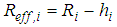where and , respectively, are the geometric radius of surface and the radial distance of surface to the pivot point of the articulated slider, respectively,

Ÿ the four friction coefficients and

Ÿ the four displacement capacities

The associated four relative motions are of plate 1 relative to plate 0, of the slider relative to plate 1, of plate 3 relative to the slider and of plate 4 relative to plate 3 whereby the total bearing displacement becomes

The vertical load ( acceleration of gravity, structural mass) on the bearing is assumed to be constant and uniformly distributed on concave plate 4 to guarantee proper functioning of the kinematics of the triple FP. The variations of the vertical load due to the small vertical acceleration of the building when the slider moves towards one side of the bearing are neglected as the focus of the study under consideration is the isolation assessment of the isolator in horizontal direction.

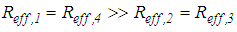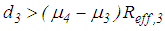
The usual design of the triple FP according to [31, 32] is given by and 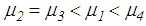in order to ensure that relative motion initiates on surfaces 2 and 3 with low friction which is followed by increasing friction characteristics when sliding also occurs on surfaces 1 and 4 and is finalized by a stiffening effect at reduced friction when concave slide plates 1 and 3 contact the restrainers of concave plates 0 and 4 whereby only the articulated slider assembly works. This behaviour is achieved when the design of the triple FP satisfies the conditions 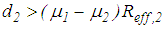, and

2.2. Properties of Triple Friction Pendulum

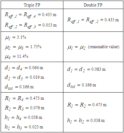
The aim of the present study is to assess the isolation performance of the triple FP as it is originally designed and published in the literature [31, 32]; the friction coefficients used in the present study represent the average values of the identified values given in [32]. This triple FP represents a mock-up triple FP whereby the effective radii 1 and 4 and consequently the isolation time period are rather small. In order to guarantee a fair comparison with the non-adaptive double FP, the effective radii 1 and 2 of the double FP and consequently its isolation time period are equal those of the triple FP. Table 1 shows the relevant parameters including the total displacement capacity (without the small influence of rotation). The vertical load kN on the bearing due to the structure also corresponds to that given in [32] that leads to a surface pressure of 54.83 MPa on the slider which represents a common value.

Table 1. Properties of Triple and Double Friction Pendulums

2.3. Non-Adaptive Double Friction Pendulum

The non-adaptive double FP consists of two concave steel plates and the rigid slider in between which is coated with a non-metallic sliding material (Figure 1(b)). The motion of the slider relative to the plate 0 is denoted as and between plate 2 and slider is whereby the total bearing motion becomes (without small influence of rotation). In order to secure a fair comparison of the isolation performances resulting from the triple and double FPs, the isolation frequency of the double FP is selected to be equal the lower isolation frequency of the triple FP. Hence, the effective radii of the double FP and are equal the effective radii of the two concave plates 0 and 4 of the triple FP (Table 1). Furthermore, total bearing displacement of the double FP is equal to of the triple FP to guarantee equal displacement capacities. The friction coefficients of the double FP are assumed to be equal, i.e. whereby the results due to the double FP are also valid for a single FP with double effective radius.

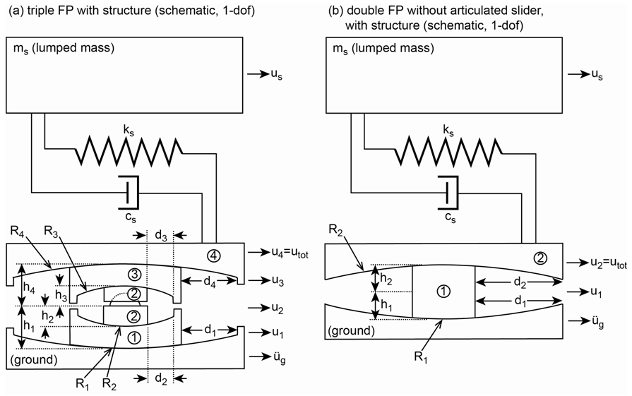Figure 1. Sketches of (a) triple friction pendulum and (b) non-adaptive double friction pendulum with structure simplified as single degree-of-freedom system (1-dof)

3. Equivalent Friction and Stiffness Coefficients

3.1. Kinematic Excitation

3.1.1. Force Displacement Trajectories

The horizontal bearing force of the triple FP is the sum of the forces due to friction, effective radius and restrainer deformation. This force resulting from kinematic excitation at the fundamental frequency of the structure is calculated adopting the formulas for all five sliding regimes as described in [31]. The computation of is not only made for the maximum displacement amplitudes of the five sliding regimes but for various total amplitudes with =1 mm, increment mm and . 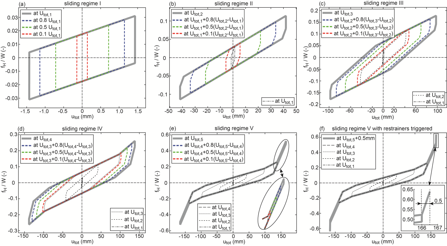The force displacement trajectories resulting from the maximum displacement amplitudes of sliding regime are depicted in Figures 2(a-e) by the thick lines in grey; the thin dashed lines in red, green and blue represent the force displacement trajectories due to three selected that are smaller than of the corresponding sliding regime. For the sake of completeness, the force displacement trajectory for 0.5 mm restrainer deformation, i.e. mm, is also shown (Figure 2(f)). Notice that the force displacement trajectories plotted in Figure 2 slightly differ from those depicted in figure 4 of [32] because the force displacement trajectories shown figure 4 of [32] are computed with , and identified for each sliding regime itself which yields different and for the five sliding regimes. It is also underlined that the force displacement trajectories depicted in Figure 2 differ from those shown in [31] because the force displacement trajectories of [31] are computed for and

Figure 2. Force displacement trajectories resulting from kinematic excitation

3.1.2. Equivalent Friction and Stiffness Coefficients

From the force displacement trajectories resulting from all considered =1 mm, increment mm, ) the equivalent friction coefficient is numerically computed from the cycle energy of [27, 42]

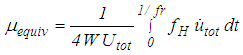(1)

where denotes the frequency of and is the total bearing velocity; the equivalent stiffness coefficient is numerically derived from the elastic energy of [27, 42]

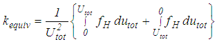(2)

3.1.3. Discussion

The obtained energy equivalent coefficients are plotted in Figures 3(a, b) versus the total amplitudes of all computed force displacement trajectories. The following observations can be made (readers are referred to [31] for detailed description of the sliding regimes of the triple FP):

Ÿ Sliding regime I: relative motion only occurs on sliding surfaces 2 and 3 with equal radii and friction coefficients (Figure 2(a)) [31]. This explains the findings

Ÿ Sliding regime II: relative motion occurs on surfaces 1, 2 and 3 (Figure 2(b)) [31]. The resulting which can be interpreted as an “average” friction coefficient is therefore greater than but smaller than while is dominated by due to

Ÿ Sliding regime III: besides sliding on surfaces 1, 2 and 3 sliding is also triggered on surface 4 [31]. The resulting force displacement trajectory is dominated by simultaneous sliding on surfaces 1, 2 and 3 with slope and all surfaces 1 to 4 with slope (Figure 2(c)). turns out to be significantly smaller than because the entire sliding motion is split into simultaneous sliding on surfaces 1, 2 and 3 and simultaneous sliding on all surfaces 1 to 4. Therefore is between and

Ÿ Sliding regime IV: sliding on surface 1 is stopped by its restrainer which evokes a stiffening effect in the force displacement trajectory for (Figure 2(d)) whereby the decreasing trend of levels off (Figure 3(b)) [31]. Since simultaneous sliding on surfaces 1 and 4 dominates the force displacement trajectory of sliding regime IV (Figure 2(d)), increases within sliding regime IV towards but is significantly smaller than because of (Figure 3(a)).

Ÿ Sliding regime V: sliding on surfaces 1 and 4 are stopped by their restrainers while sliding continuous on sliding surfaces 2 and 3. This evokes the stiffening behaviour at very small friction for (Figure 2(e)). As a result, increases while decreases in sliding regime V.

Figure 3. (a) Cycle energy equivalent friction coefficient and (b) elastic energy equivalent stiffness coefficient as function of total displacement amplitude identified from kinematic excitation

3.2. Force Excitation

In order to compute the energy equivalent friction and stiffness coefficients for force excitation, first, the coupled equations of motion of the isolated structure and all bearing plates of the triple FP for ground acceleration input are derived (section 3.2.1), then the input acceleration is described (section 3.2.2) and, finally, the obtained results are discussed (section 3.2.3).

3.2.1. Coupled Non-Linear Equations of Motion

The equation of motion of the structure with ground acceleration as excitation input becomes

(3)

where denotes the relative structural acceleration, is the modal mass ( acceleration of gravity), is the viscous damping coefficient with damping ratio is the stiffness coefficient, and and respectively, represent the relative displacement and relative velocity, respectively, between the structure and concave plate 4 of the triple FP (Figure 1(a)). The excitation force due to the ground acceleration is given by the d’Alembert term on the right side of (3) whereby the total acceleration of the structure becomes . The structural stiffness 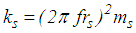is selected such that the fundamental frequency of the non-isolated structure is two times higher than the lower isolation frequency of the triple FP

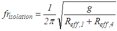(4)

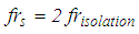(5)

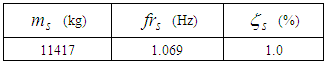
Equation (4) yields Hz representing a typical value of non-isolated structures that require base isolation. All relevant structural properties are given in Table 2 where the given mass corresponds to the mass of the structure supported by one pendulum.

Table 2. Structural properties

The formulation of the equation of motion for concave plate 4 with mass yields (Figure 1(a))

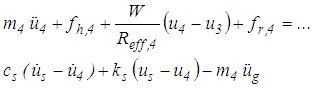(6)

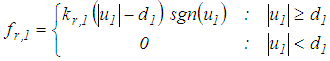
where denotes the relative acceleration of represents the friction force of surface 4, is the stiffness due to the effective radius of concave plate 4 and is the restrainer force of concave plate 4. is modelled by the hysteretic friction force model where the pre-sliding regime is modelled by a stiffness force [43, 44]

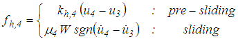(7)

The pre-sliding stiffness is selected to be 5e2 times greater than the stiffness due to the effective radius, i.e. 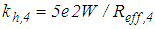, represents the signum function and is the relative velocity between the plates 4 and 3. The force of the restrainer is modelled as a linear stiffness force that is only triggered when plate 3 is in contact with the restrainer of plate 4

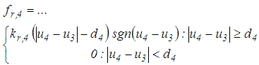(8)

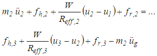
where the restrainer stiffness is selected to be 1e2 times greater than For the concave slide plate 3 with mass the equation of motion is

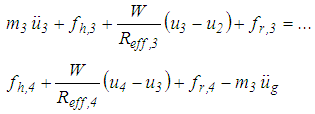(9)

where is the relative acceleration of and and respectively, represent the hysteretic friction force and restrainer force, respectively, that are formulated analogically with equations (7, 8). The equation of motion for the slider mass has the same form as for

(10)

where denotes the relative acceleration of the slider and and respectively, are given analogically with equations (7, 8). The equation of motion of concave plate 1 with mass and relative acceleration becomes

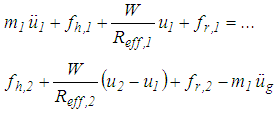(11)

where and respectively, are given as follows

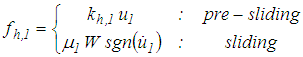(12)

(13)

because is the displacement of plate 1 relative to plate 0 (Figure 1(a)). It must be added that and are assumed and that the values of and are calculated based on the geometrical data given in [32] assuming steel as material.

3.2.2. Dynamic Simulation

The coupled non-linear differential equations of motion are solved in the time domain in Matlab/Simulink® using the solver ode15s(stiff/NDF) with maximum relative tolerance of 1e-3 and variable step size with upper bound of 1e-5 s.

3.2.3. Ground Acceleration

In order to trigger all sliding regimes of the triple FP under force excitation step by step, the ground acceleration is assumed to be a sinusoidal function with linearly increasing amplitude and frequency (Figure 4(a)). The resulting relative displacements show that the restrainer of plate 0 is first triggered, then the restrainers of plate 0 and 4 are triggered during one cycle of vibration and finally all four restrainers of plates 0, 1, 3 and 4 are triggered during one cycle of vibration (Figure 4(b)). Then, the simulation is stopped because the full displacement capacity of the bearing is depleted.

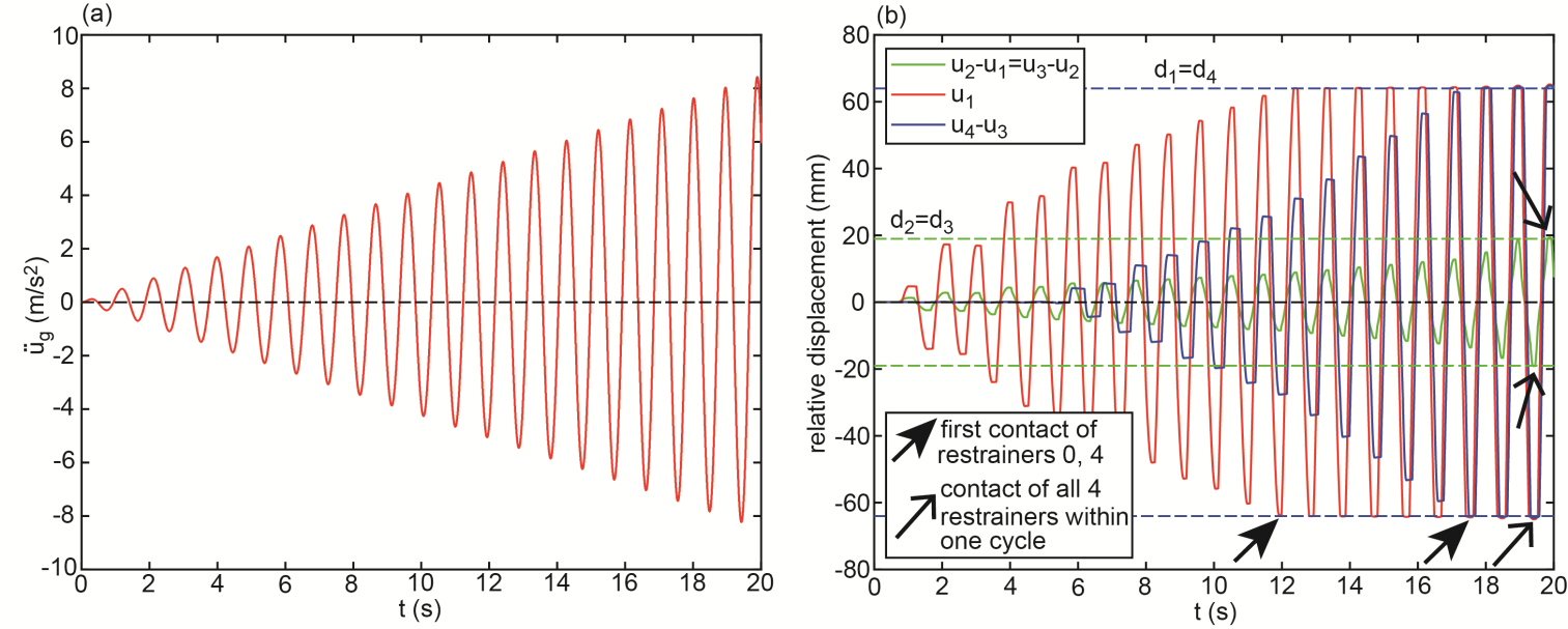Figure 4. Behaviour of triple FP under force excitation: (a) introduced ground acceleration, (b) relative bearing displacements

3.2.4. Discussion

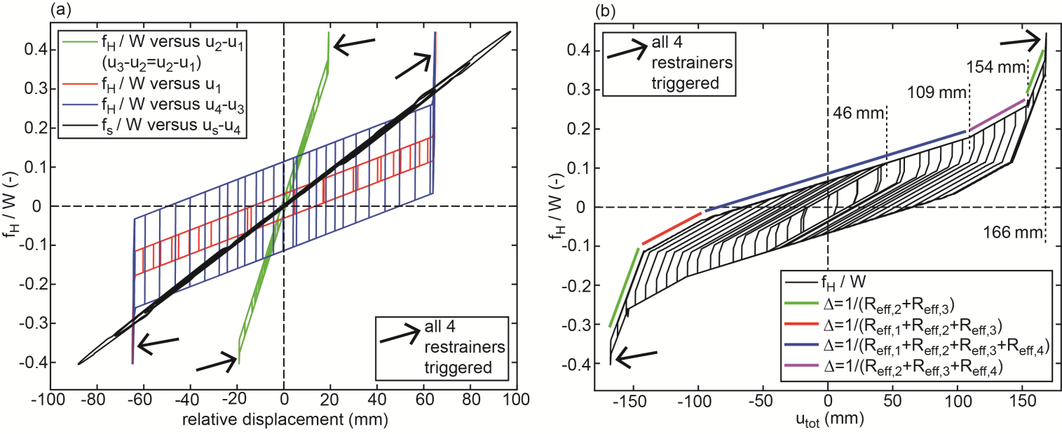
The horizontal forces of masses 1, 2, 3, 4 and the visco-elastic structural force are equal at every time instant

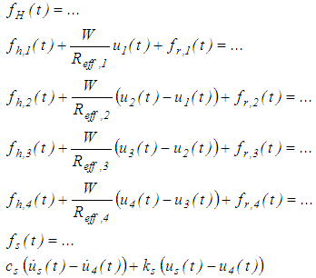(14)

The corresponding force displacement trajectories are not congruent, see Figure 5(a), because of the different relative displacements and (see also Figure 4(b)). Figure 5(b) plots versus the total bearing displacement which can be compared with the force displacement trajectories from kinematic excitation (Figure 2). The main difference observed is that when sliding is also triggered on surface 4 see Figure 4(b)), simultaneous sliding takes place on all four sliding surfaces which is confirmed by the slope of the force displacement trajectory (normalized by ) of

Figure 5. Behaviour of triple FP under force excitation: (a) horizontal force versus relative displacements of triple FP and primary structure, (b) horizontal force versus total displacement

This observation reveals that the triple FP installed between foundation and structure and excited by ground acceleration behaves different than for kinematic excitation as described in [31]. In order to double-check this finding, half a cycle from sliding start to sliding stop is investigated in detail. Figure 6(a) depicts the four relative bearing displacements as function of time that are normalized when sliding initiates on surfaces 2 and 3. The corresponding force displacement trajectories of the same time interval are plotted in Figure 6(b). When sliding only occurs on surfaces 2 and 3, their horizontal forces are balanced by the pre-sliding stiffness forces and 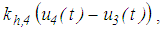respectively, of surfaces 1 and 4, respectively. Sliding on surface 1 initiates when the relative motions 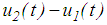and 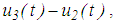respectively, are that large that the sum of increased stiffness forces due to the effective radii of surfaces 2 and 3 and the constant friction force balance the friction force of surface 1, that is

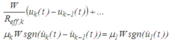(15)

where for the slider and for concave plate 3, which is highlighted by the circle symbol in Figures 6(a, b). With further increased relative motions , and , respectively, the friction force is balanced by the sum of the stiffness force due to and friction force of surface 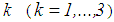whereby sliding starts on surface 4 (diamond symbol in Figures 6(a, b)). All relative motions stop at the same time instant when all four hysteretic friction forces get back into their pre-sliding regimes (star symbol in Figures 6(a, b)).

Figure 6. Simultaneous sliding on surfaces 1, 2, 3 and 4: (a) relative displacements as function of time and (b) horizontal force versus relative displacements

Comparing the equivalent friction and stiffness coefficients due to forced excitation (Figures 7(a, b)) with those resulting from kinematic excitation (Figures 3(a, b)) shows:

Ÿ The total displacement amplitudes of sliding regimes I to V are shifted to greater values; notice that for the computation of the force displacement trajectories due to kinematic excitation (section 3.1) correspond to those given in [31].

Ÿ The values of are almost the same as resulting from the force displacement trajectories due to kinematic excitation but are shifted to larger for the reason mentioned above and also significantly decreases when sliding regime V is activated.

Ÿ The softening effect of is slightly bigger due to the simultaneous sliding on all four surfaces whereby gets close to and the stiffening effect due to sliding regime V is less pronounced.

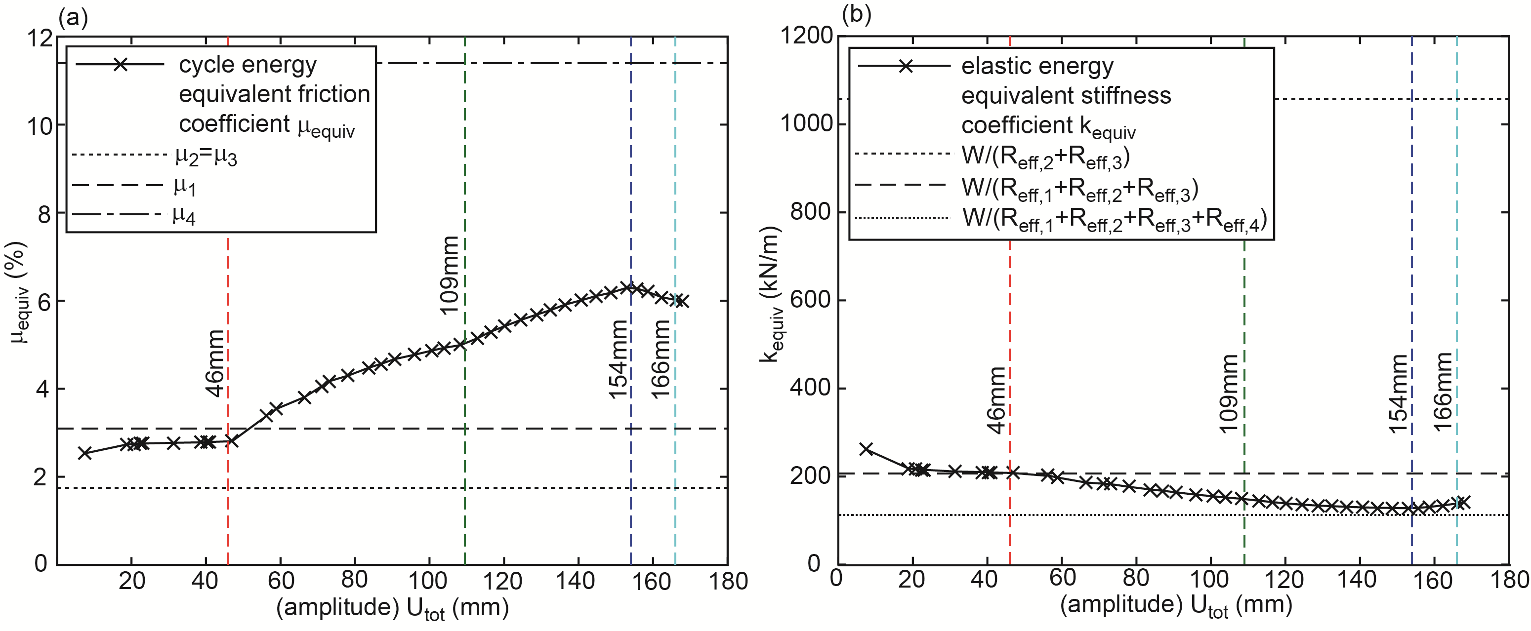Figure 7. (a) Cycle energy equivalent friction coefficient and (b) elastic energy equivalent stiffness coefficient depending on total displacement amplitude and due to force excitation

4. Isolation Performance

Section 4 compares the isolation performance of the triple FP with that of the non-adaptive double FP with equal radii and equal friction coefficients. To guarantee a fair comparison the effective radii of the double FP are equal those of concave plates 0 and 4 of the triple FP (Table 1). Since the equivalent friction and stiffness coefficients of the triple FP depend on the bearing displacement amplitude, the isolation performance of the triple FP is assessed for various PGA values of several earthquakes to operate the triple FP within all its sliding regimes (section 4.1). The equal friction coefficients of the double FP are selected so that the restrainer deformation of the double FP at maximum PGA value is approx. equal that of the triple FP at maximum PGA value (section 4.2). The simulations are evaluated in terms of extremes of absolute acceleration and drift of the structure (section 4.3) and discussed in section 4.4.

4.1. PGA-scaled Ground Acceleration Time Histories

The simulations are performed with the ground acceleration time histories of the El Centro North-South (NS) earthquake, the El Centro East-West (EW) earthquake, the Loma Prieta earthquake, the Kobe earthquake and the Northridge earthquake. In order to operate the triple FP within all its sliding regimes the ground acceleration time histories are scaled by the following PGA-values in m/s²

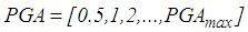(16)

where the maximum PGA value is chosen so that the maximum restrainer deformation of the triple FP is less than 1 mm. Due to the different frequency contents of the considered earth-quakes becomes 7.8 m/s² for the El Centro NS earthquake, 4.9 m/s² for the El Centro EW earthquake, 3.2 m/s² for the Loma Prieta earthquake, 3.82 m/s² for the Kobe earthquake and 6.45 m/s² for the Northridge earthquake.

4.2. Friction Coefficient of Double Friction Pendulum

The friction coefficients of the double FP are selected so that the restrainer deformation of the double FP is less than 1 mm at This ensures that displacement capacities of both the double and triple FPs are fully depleted at . The resulting friction coefficients are for the El Centro NS earthquake, for the El Centro EW earthquake, for the Loma Prieta earthquake, for the Kobe earthquake and for the Northridge earthquake. In addition, all simulations are also performed with assuming a double FP with one friction coefficient.

4.3. Evaluation Criteria

The isolation performance is assessed by the commonly adopted two criteria [24, 26]:

Ÿ extreme of the absolute structural acceleration and

Ÿ extreme of the structural drift where for the triple FP and in case of the double FP (Figures 1(a, b)).

4.4. Results

4.4.1. Simulation Tool

For the simulations of the structure with triple FP the coupled non-linear differential equations de-scribed in section 3.2.1 are solved in Matlab/Simulink® (solver ode15s(stiff/NDF), maximum relative tolerance 1e-3, variable step size with upper bound of 1e-5 s) for the PGA-scaled ground accelerations of the five considered earthquakes. For the simulations of the structure with double FP, the equations of motion are reformulated for the two degrees of freedom and of the double FP.

4.4.2. Absolute Acceleration and Drift of Structure

The simulation result of and for the El Centro NS earthquake are depicted in Figures 8(a, b). It is observed that and show the same trend as function of PGA which also applies to the simulation results of the other four earthquakes. This is explained by the fact that the structure is modelled as a single degree-of-freedom system which is the common approach when the isolation frequency is significantly below the natural frequency of the structure [45, 46] (Fig. 1). Therefore, Figures 9(a, b) and 10(a, b) only depict resulting from the simulations of the El Centro EW, the Loma Prieta, the Kobe and the Northridge earthquake.

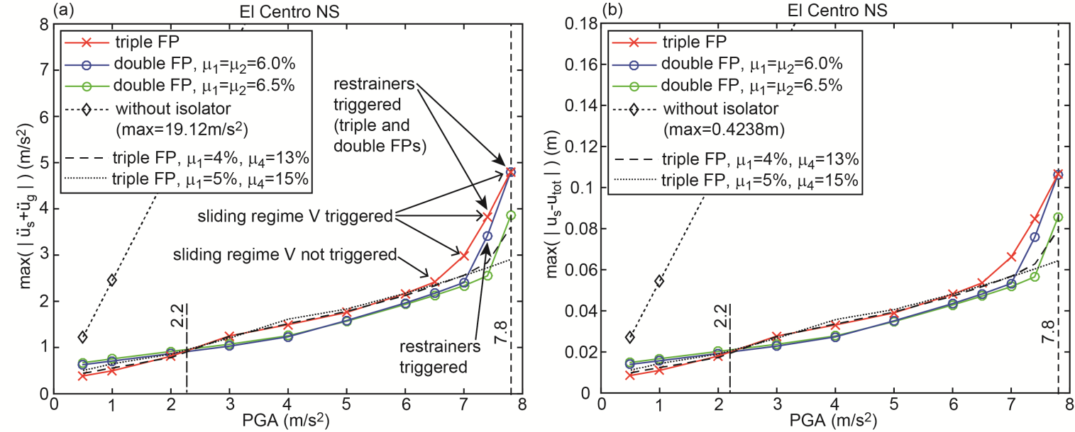Figure 8. (a) Extreme of absolute acceleration of structure and (b) extreme of total drift of structure due to triple FP, double FP and without isolator due to El Centro NS earthquake

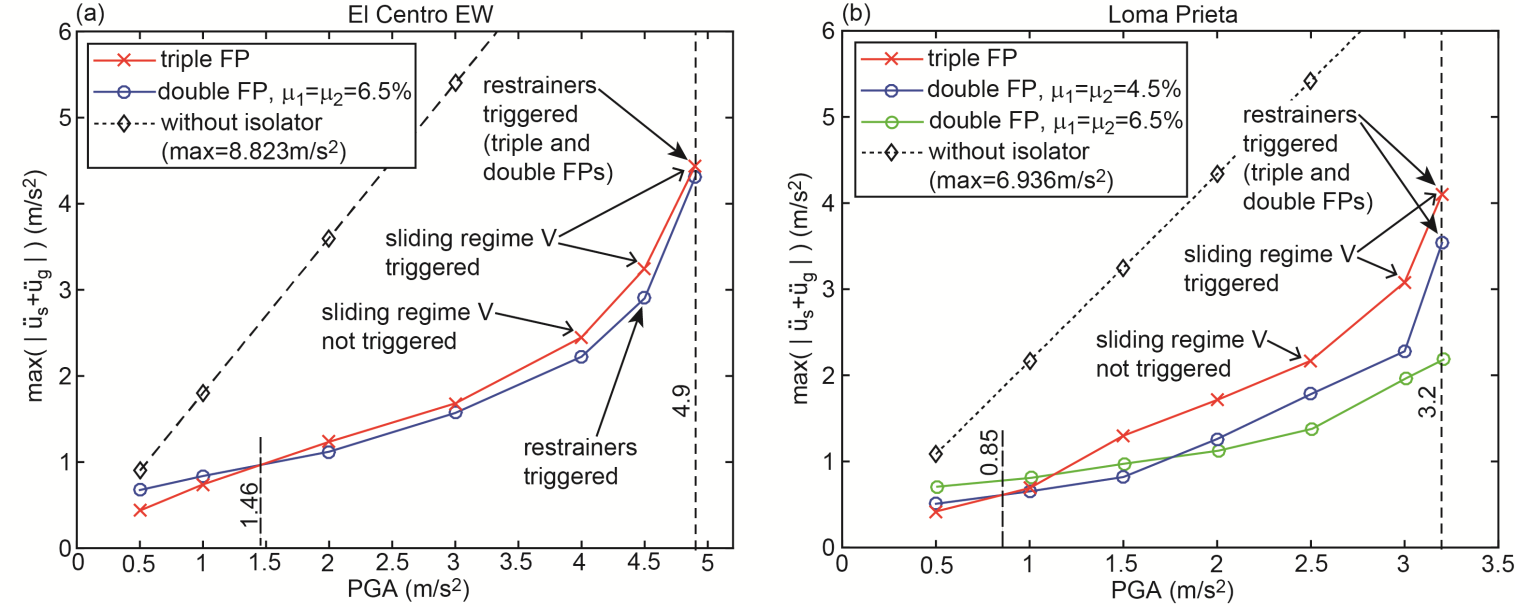Figure 9. Extreme of absolute acceleration of structure due to triple FP, double FP and without isolator due to (a) El Centro EW and (b) Loma Prieta earthquakes

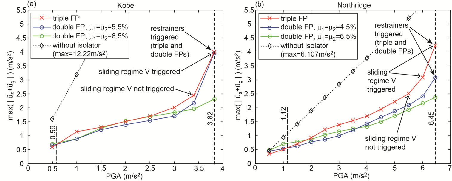Figure 10. Extreme of absolute acceleration of structure due to triple FP, double FP and without isolator due to (a) Kobe and (b) Northridge earthquakes

4.4.3. Triple Friction Pendulum Compared with Double Friction Pendulum

The numerical results of all considered earthquakes and PGA values reveal:

Ÿ The triple FP performs better at small the PGA values: PGA<2.2 m/s² for the El Centro NS, PGA<1.46 m/s² for El Centro EW, PGA<0.85 m/s² (<1.12 m/s² for 6.5%) for the Loma Prieta, PGA<0.59 m/s² (<0.63 m/s² for 6.5%) for the Kobe and PGA<1.12 m/s² (<1.83 m/s² for 6.5%) for the Northridge earthquake.

Ÿ The double FP outperforms the triple FP for PGA values greater than the values given above.

Ÿ The isolation performances of both FPs at are almost equal because triggers approx. the same restrainer deformation (see section 4.1).

Ÿ The double FP with 6.5% friction (plotted in green) performs best because the higher friction reduces the bearing relative motion whereby restrainers are not triggered at

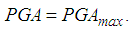
4.4.4. Triple Friction Pendulum with Different Friction Coefficients

The fact that the double FPs perform significantly better for most PGA values than the triple FP with and may be caused by suboptimal tunings of and of the triple FP; notice that and represent the experimentally identified mean values presented in [32]. Since the good results of the double FPs for the El Centro NS earthquake are obtained with significantly greater friction coefficients than 3.1%, two other triple FPs with increased friction coefficients, i.e. and and and are also computed. The results, which are included in Figures 8(a, b), demonstrate that increased friction coefficients and do hardly improve the isolation performance of the triple FP for most PGA values except in the vicinity of due to the greater friction coefficients that reduce the total bearing motion whereby the restrainer deformation becomes smaller in case of and and becomes zero for and It should be added that increased friction coefficients in case of the double FP would also avoid the activation of the restrainers whereby also the isolation results of the double FP at PGA values close to would be improved.

4.4.5. Impact of Sliding Regime V

The results depicted in Figures 8(a, b)-10(a, b) clearly point out that the isolation performance of the triple FP deteriorates in the vicinity of The double-check of all force displacement trajectories of all simulations reveals that this coincides with the activation of sliding regime V (Figures 11(a, b, c)) that is characterized by significantly increased stiffness and significantly reduced friction. The combination of increased stiffness and reduced friction:

1.evokes the deterioration of the isolation because increased stiffness is equivalent to reduced isolation time period which would require increased friction to compensate for the isolation deterioration, and

2.cannot reduce the bearing displacement capacity demand since the stiffening behaviour is offset by the reduced friction which is confirmed by the equal restrainer deformations at of the triple and double FPs with equal to (Figures 11(d, e, f)).

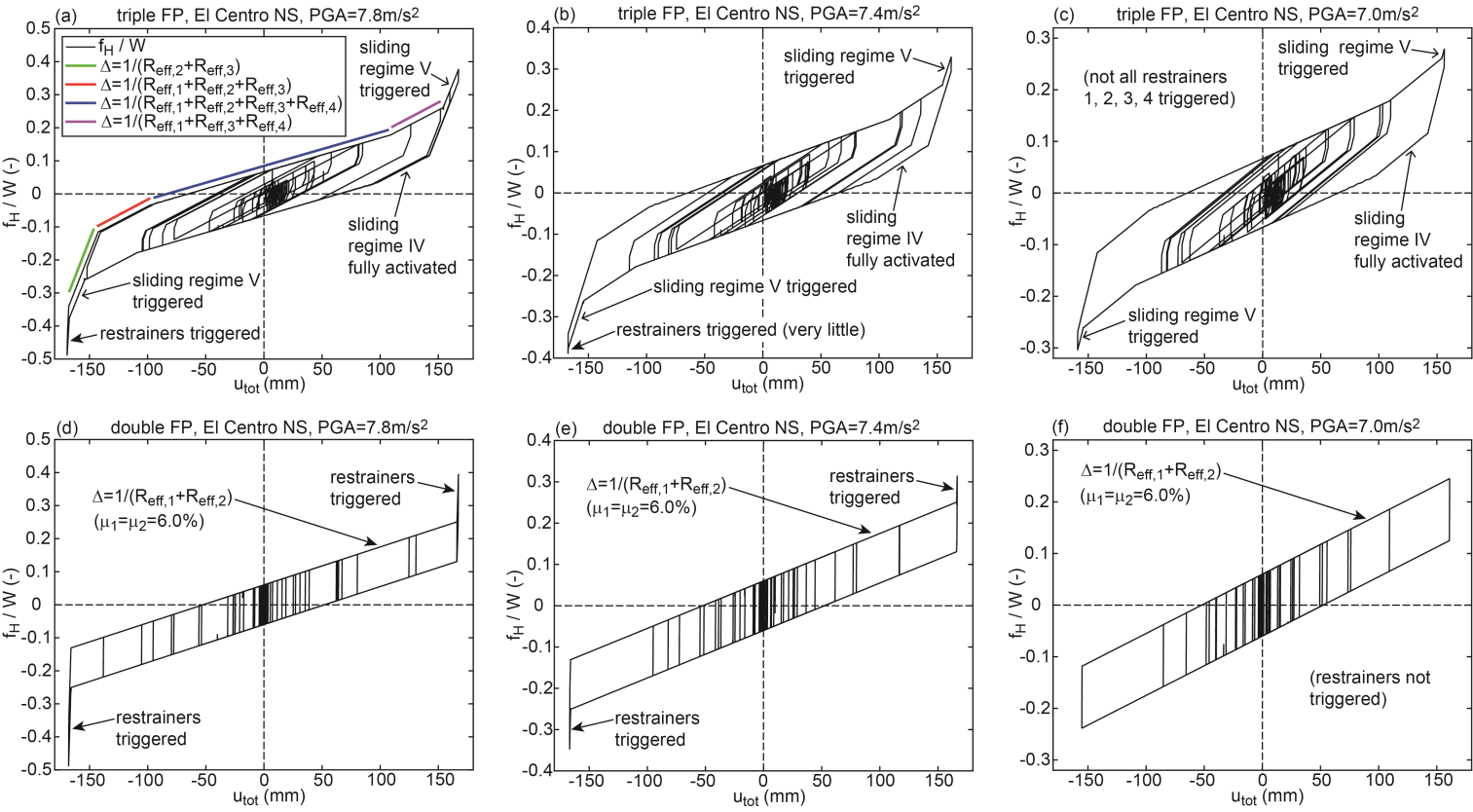Figure 11. Horizontal force versus total displacement of triple FP due to El Centro NS for (a) PGA=7.8 m/s2, (b) PGA=7.4 m/s2, (c) PGA=7.0 m/s2 and of double FP due to El Centro NS for (d) PGA=7.8 m/s2, (e) PGA=7.4 m/s2 and (f) PGA=7.0 m/s2

In contrast to sliding regime V sliding regime IV does not lead to a deterioration of the isolation performance despite the small stiffening effect of sliding regime IV as observed in Figure 12(a) because the activation of sliding regime generates a further increase of the equivalent friction coefficient as depicted in Figures 3(a) and 7(a). Figures 12(b-f) show that the force displacement trajectories of the triple FP at medium to small PGA values is dominated by sliding regimes II and III while sliding regime I is only relevant at PGA=0.5 m/s² which is also seen from the values of and in Figures 3(a, b) and 7(a, b).

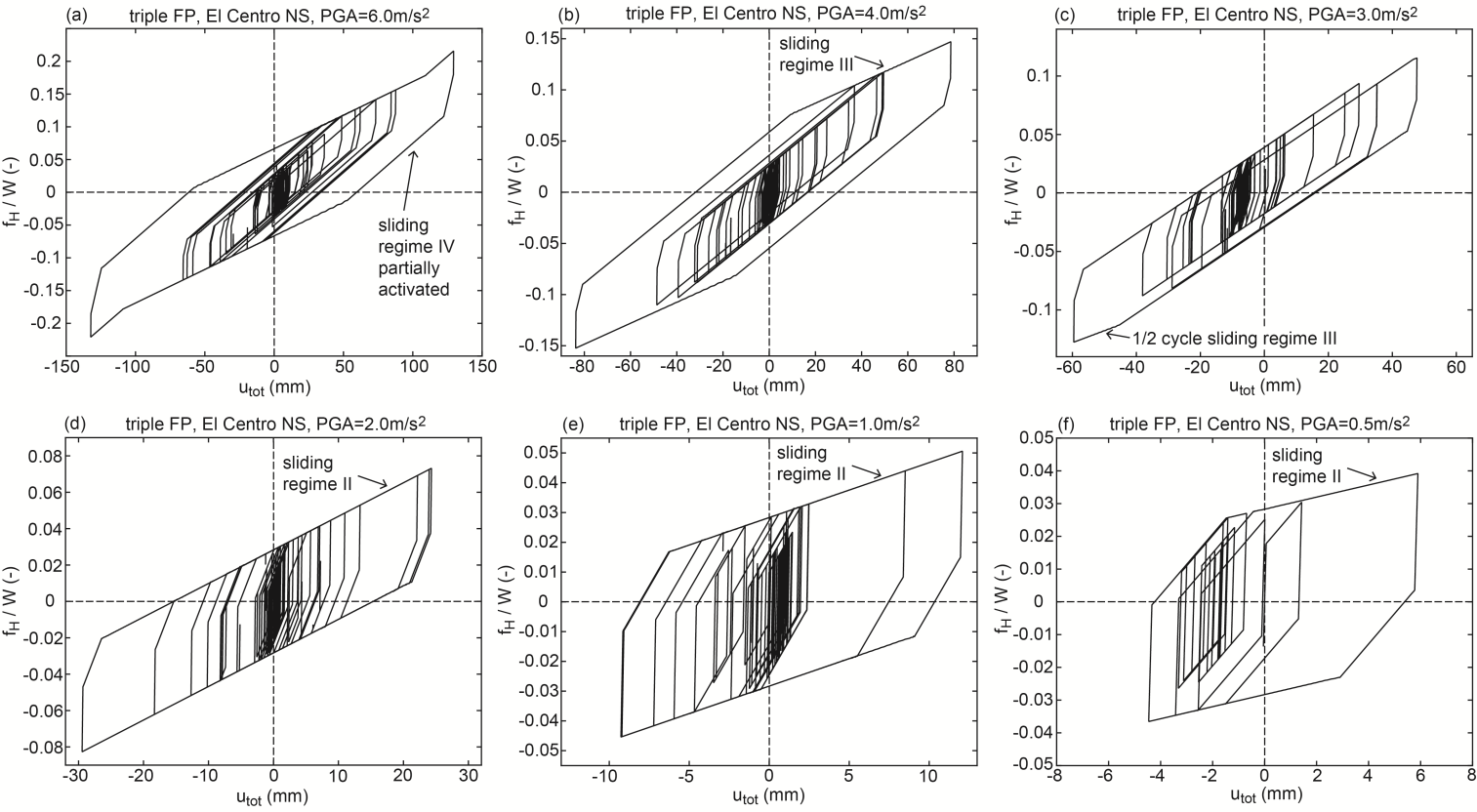Figure 12. Horizontal force versus total displacement of triple FP due to El Centro NS for (a) PGA=6.0 m/s2, (b) PGA=4.0 m/s2, (c) PGA=3.0 m/s2, (d) PGA=2.0 m/s2, (e) PGA=1.0 m/s2 and (f) PGA=0.5 m/s2

5. Friction in Proportion to Displacement Amplitude

5.1. Adaptive Friction?

As demonstrated in section 2 the equivalent friction coefficient of the triple FP increases with increasing bearing relative motion within sliding regimes II to IV which primarily determine the dynamic behaviour of the triple FP (Figure 3(a)). Also within sliding regimes II to IV the equivalent stiffness coefficient shows a decreasing trend (Figure 3(b)). Both adaptive behaviours are commonly considered to improve the isolation of the primary structure. However, the results presented in section 4 demonstrate the contrary, i.e. the conventional non-adaptive double FP outperforms the triple FP at medium to higher shaking levels at which sliding regimes II to IV are activated.

In order to better understand how friction should depend on bearing motion in order to improve structural isolation a case study is performed where the friction coefficient of the pendulum is controlled in proportion to bearing displacement amplitude which is described subsequently.

5.2. Energy Balance with Linear Viscous Damper

The goal of any damping mechanism is to maximize the cycle energy of the damping device independent of its displacement amplitude. This means that the damping device should be linear, i.e. produce linear viscous damping. In order to obtain the control law of a controlled friction device it is therefore reasonable to balance the cycle energies of a linear viscous damper and a friction damper [47, 48]

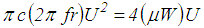(17)

where denotes the viscous damper coefficient of the linear viscous damper and harmonic excitation is assumed. Equation (17) can be interpreted as the cycle energy balance of a pendulum (without friction) with a linear viscous damper in parallel and a conventional FP. Solving (17) for the friction coefficient and omitting all constant variables yields

(18)

Furthermore, may be assumed considering that the frequency of the relative motion of the FP is in the vicinity of the isolation frequency that is given by the curvature of the FP. With this assumption it turns out that the friction coefficient should be adjusted in proportion to relative displacement amplitude [47-53]

(19)

5.3. Ideal Pendulum with Friction in Proportion to Displacement Amplitude

Ideally, a curved surface without any friction is combined with a controllable damper [54], e.g. a magnetorheological damper [27, 28, 55], to realize (19). The according real-time controlled friction force of the controllable damper becomes

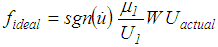(20)

where denotes the gradient of friction relative to displacement amplitude (indicated by the dashed line in red in Figure 13(a)) and is the actual displacement amplitude. The resulting force displacement characteristics including the restoring stiffness force due to the curvature are depicted in Figure 13(a) for five selected .

5.4. Real Pendulum with Passive (Lubricated) Friction and Real-time Controlled Friction

In reality, friction of curved surfaces cannot be avoided. The lowest value is obtained when the sliding surface is lubricated. Typically, the lubricated (passive, uncontrollable) friction coefficient is around 1%. The sum of the force due to lubricated friction of the FP and the controlled friction force of the controllable damper therefore becomes

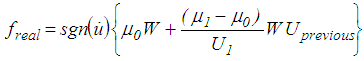(21)

Here, denotes the previous (latest) displacement amplitude as the previous value is the latest value available in real-time control [50]. The resulting force displacement trajectories due to the simulation of the Loma Prieta earthquake scaled to PGA=2 m/s² show local loops (Figure 13(b)) due to the broad band excitation of the accelerogram in contrast to the force displacement trajectories shown in Figure 13(a) that result from kinematic excitation at constant frequency and constant amplitude.

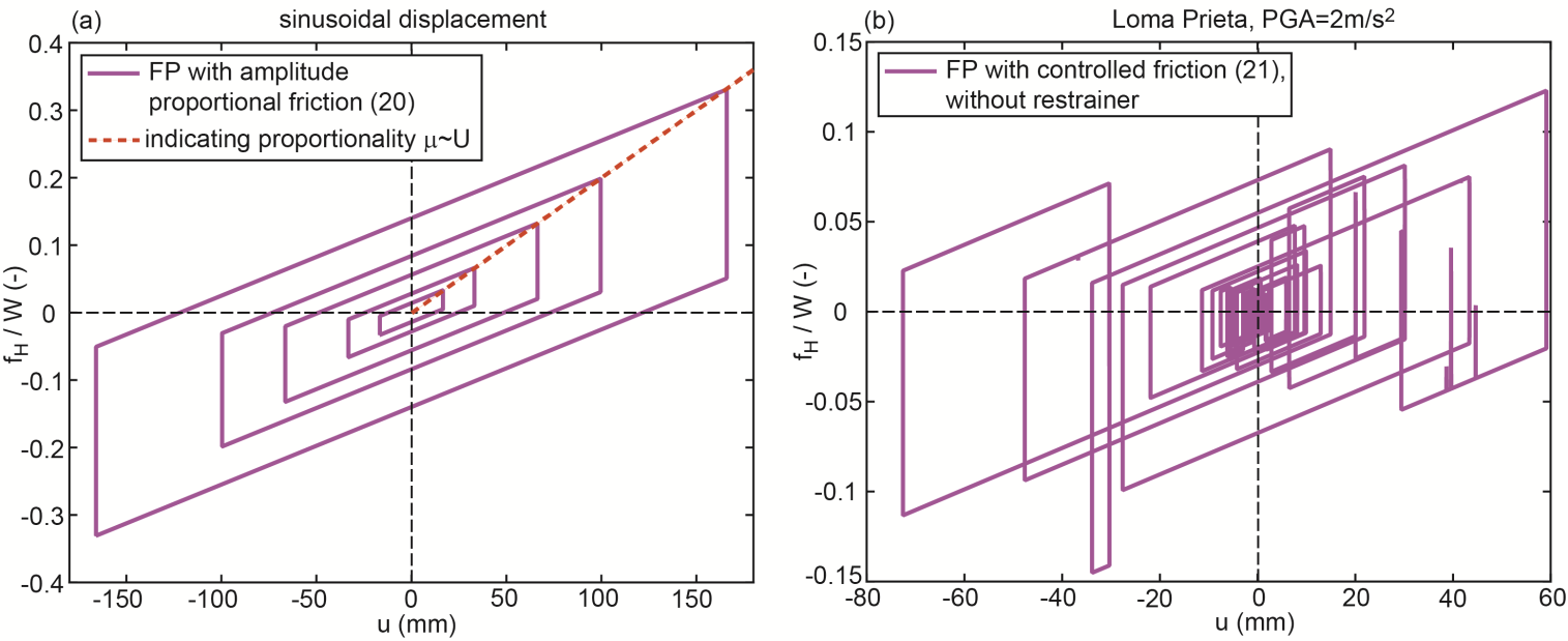Figure 13. Force displacement trajectories of (a) FP according to (20) for kinematic excitation and (b) FP according to (21) due to ground excitation

5.5. Assessment for Two Accelerograms

The isolation performance of the pendulum with lubricated (passive, uncontrollable) friction and real-time controlled friction force according to (21) is computed for the accelerograms of the El Centro NS and the Loma Prieta earthquakes. The results plotted in Figures 14(a, b) are compared to those of two double FPs without restrainers to avoid the deteriorated isolation results at PGAs in the vicinity of and to those of two triple FPs with increased friction coefficients also to avoid the worse isolation results when all restrainers are activated as seen in, e.g., Figures 8(a, b).

It is observed that the pendulum with lubricated (passive, uncontrollable) friction of 1% and a friction force that is adjusted in real-time in proportion to the previous displacement amplitude significantly outperforms all other computed double and triple FPs within the entire PGA range. The values of the absolute structural peak accelerations almost describe a straight line which means that controlling the friction force in proportion to displacement amplitude linearizes the friction damper over each cycle (the force is still a friction force, see Figure 13(b)) which is the direct result of the energy balance with the linear viscous damper (17). A linear line would be obtained if and amplitude estimation errors were not present which corresponds to the ideal pendulum with controlled friction according to (20). It is also observed that the conventional double FP generates the same isolation as approach (21) at these PGAs for which the constant friction coefficients of the conventional double FP are correctly tuned to the bearing displacement amplitude which is triggered when the peak of the structural acceleration occurs. The slightly better isolation result of the double FP with 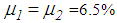for the Loma Prieta accelerogram scaled to PGA=2.5 m/s² is caused by the fact that the friction coefficient of (21) is controlled in proportion to which is not the actual amplitude whereby small real-time tuning errors in the actual friction force (21) are present.

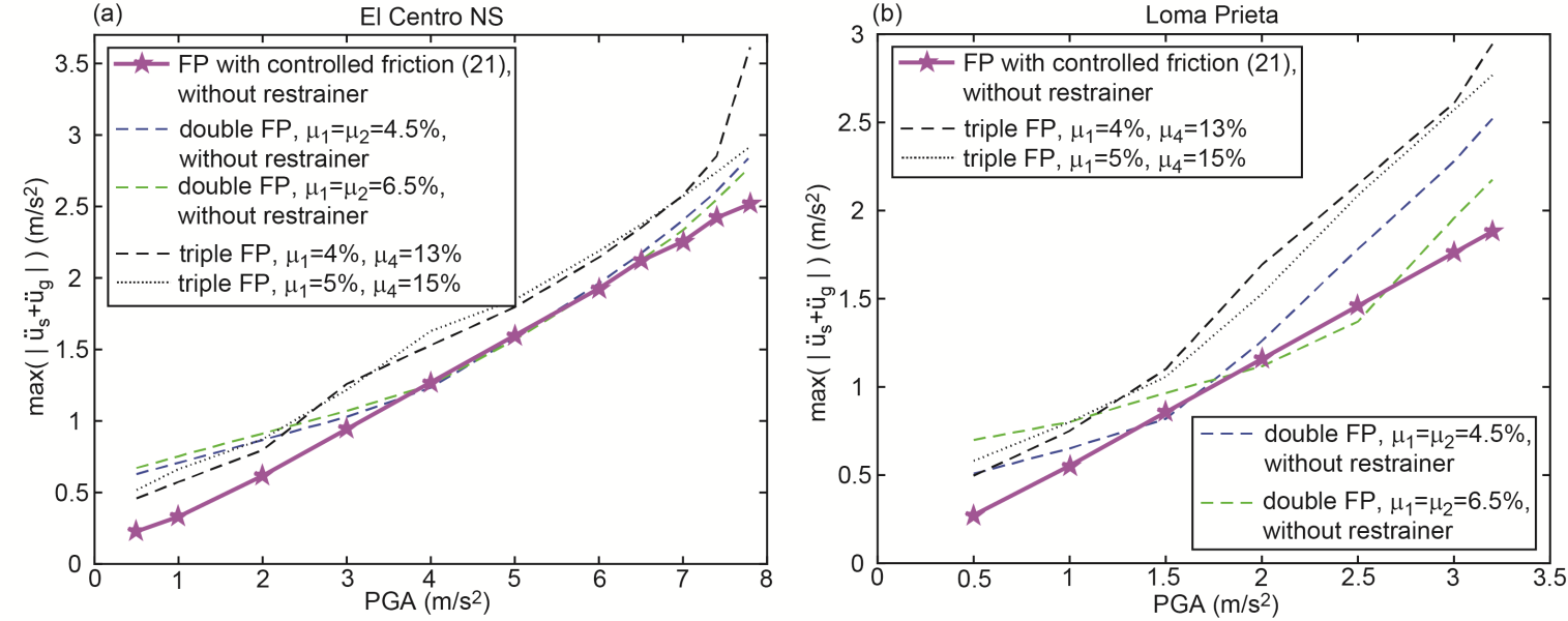Figure 14. Performance of single FP with friction controlled in real-time in proportion to displacement amplitude for (a) El Centro NS and (b) Loma Prieta earthquakes compared with double FPs without restrainers and best performing triple FPs

6. Conclusions

The triple friction pendulum (FP) is well-known for its adaptive friction and stiffness properties that depend on its sliding regimes and bearing displacement amplitude, respectively, and consequently on peak ground acceleration (PGA) of the considered accelerogram. This paper therefore assesses the isolation performance in terms of absolute structural peak acceleration as function of various PGAs ranging between very small values up to the maximum value at which the full displacement capacity of the triple FP is used. The resulting isolation results demonstrate that the low friction of the articulated slider assembly is beneficial as it triggers relative motion in the bearing at small PGAs (<20% of its maximum) while the conventional non-adaptive double FP with same curvature outperforms the triple FP for all other PGAs. It is also observed that sliding regime V evokes a strongly deteriorated isolation due to the increased stiffness that reduces the isolation time period. In addition it is found that the increased stiffness of sliding regime V cannot reduce the displacement capacity of the triple FP because it is accompanied by reduced friction; the displacement capacity could be reduced by the combinations of increased stiffness and maintained friction or increased friction and maintained stiffness.

Based on the finding that the displacement (position) dependent friction of sliding regimes II to IV of the triple FP is not beneficial for enhanced structural isolation a pendulum is presented whose friction coefficient is controlled in proportion to bearing displacement amplitude. This approach is derived from the energy balance between linear viscous and friction dampers and requires the adoption of a controllable damper that works in parallel with the curved surface. To minimize the uncontrollable friction of the isolator the curved surface is assumed to be lubricated. The results demonstrate that the FP with friction controlled in proportion to displacement amplitude significantly enhances the isolation of the structure. Hence, displacement amplitude proportional friction is seen as the objective function for the future development of adaptive pendulums based on passive mechanisms without the adoption of control devices.

ACKNOWLEDGEMENTS

The authors gratefully acknowledge the financial support of MAURER SE, Munich, Germany.

REFERENCES