John N. Karadelis, Lei Zhang
Department of Civil Engineering, Architecture and Building, Coventry University, Coventry, UK
Correspondence to: John N. Karadelis, Department of Civil Engineering, Architecture and Building, Coventry University, Coventry, UK.
| Email: |  |
Copyright © 2015 Scientific & Academic Publishing. All Rights Reserved.
This work is licensed under the Creative Commons Attribution International License (CC BY).
http://creativecommons.org/licenses/by/4.0/

Abstract
The main aim of this article is to simulate the tensile behaviour of steel fibre reinforced concrete (SFRC) by using the finite element analysis (FEA) code, ABAQUS. A simple, direct, discrete modelling plan is proposed based on pioneering theoretical work by others. A bilinear stiffness degradation model for steel fibre was considered to simulate the softening portion of the load - crack mouth opening displacement curve. A corresponding sensitivity study was conducted and recommended values for all relative parameters were established. Overall, the simulated results projected the main features of the tensile behaviour of steel fibre reinforced concrete (SFRC) beam specimen satisfactorily.
Keywords:
SFRC Simulation, FEA, ABAQUS, Stiffness degradation, Crack
Cite this paper: John N. Karadelis, Lei Zhang, On the Discrete Numerical Simulation of Steel Fibre Reinforced Concrete (SFRC), Journal of Civil Engineering Research, Vol. 5 No. 6, 2015, pp. 151-157. doi: 10.5923/j.jce.20150506.04.
1. Introduction
Fibre reinforced composite (FRC), a relatively new concept in civil engineering materials, was firstly introduced in 1874. The composite model was conventionally considered as a two-component system, namely the fibre and the matrix [1]. As one eminent example of FRC, steel fibre reinforced concrete (SFRC) combines conventional concrete and steel fibres together. This way a high mechanical performance can be achieved under tensile load due to both high tensile strength of the steel fibre and interactions between matrix and fibres.A number of experiments incorporating SFRC have been carried out by researchers around the world. Basic fracture characteristics were fully researched by [2-4].Meanwhile, the numerical simulation of SFRC has been given more attention in recent years. The softening behaviour of SFRC is a vital feature in FEA simulation. Abdalla and Karihaloo [5] and Slowikand his co-workers [6] proposed several different models, obtaining satisfactory results. The researchers focused mainly on how to introduce steel fibre into the concrete model. Luccioni [7] Radtke [8] and Vanalli [9] proposed different methods to answer this problem, gaining acceptable results. It is worth noting that Luccioni and his co-workers proposed a homogenization approach to model SFRC based on modified mixture theory. Meanwhile, Radtke and hisassociates presented a model for failure analysis of SFRC with discrete treatment of steel fibres.The main task of this article is to establish an effective methodology to simulate the mechanical behaviour of steel fibre reinforced concrete under three-point-bending (3PB) conditions. The simulation is mainly focused on modelling the SFRC, the randomly distributed steel fibres in the matrix. Lin [10] conducted a series of experiments as part of his doctoral studies at Coventry University and obtained some good quality results. The latter were used to calibrate and validate this work. Several key factors associated with modelling, such as modelling techniques, critical parameters and solution procedures are likewise reported and justified here.
2. Material Models
2.1. Concrete Matrix
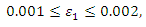
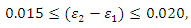
Three different models specifically designed for concrete material are catered for in ABAQUS 6.10. These are: (a). Concrete Smeared Cracking, (b). Cracking Model for Concrete and (c). Concrete Damaged Plasticity [11].However, neither the Concrete Smeared Cracking nor the Concrete Damaged Plasticity mentioned above is suitable as they both lack the ability to fully represent the constitutive relationship of concrete. This leaves us with the Cracking Model for Concrete to be employed in the FEA model.Tension stiffening is an important aspect in the simulation of reinforced concrete. The bilinear tension stiffening model for concrete proposed by Wittmann [12] is adopted. The shadowed area in Figure 1 is equal to fracture energy,  for Mode I.A range of values of two coordinates
 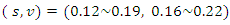 are recommended by Wittmann.
 | Figure 1. Bilinear tension softening model |
According to basic linear fracture mechanics theory, the relationship between critical stress intensity factor,  and fracture energy,
  is given by:
 | (1) |
Where:  is fracture energy,
  is critical stress intensity factor,
  is tensile strength and
  is displacement. The
  obtained from the experiment can be converted to
  as per equation (2).
 | (2) |
The shear retention model defines the relationship between the shear stiffness and crack opening (ABAQUS, 2010). As the experimental investigation carried out was a purely Mode I (opening) failure, shear retention has limited effects on the behaviour of the model. However, shear retention is necessary in the cracking model for concrete. In practice, a simple linear model can be assigned, for simplicity.In this case, the Young's modulus of the matrix can be given by the following expression [13]:  | (3) |
Where,  is volume fraction of steel fibre,
  and
and  are the Young's moduli of the composite, fibre and concrete matrix respectively. Hence the Young's modulus of the matrix can be calculated as:
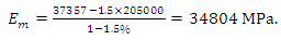 | (4) |
The density of the matrix can be assigned to a typical value: 2400 kgm-3. Other parameters needed have been taken from the experimental work and are reported in Table 1.Table 1. Material parameters employed in the FEA model
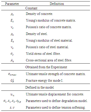 |
| |
|
2.2. Steel Fibre
A variety of constitutive models for steel are available today. Here, the basic elastic-perfectly plastic model is adopted due to its adequate accuracy and simplicity. Poisson's ratio is set to 0.3. A realistic density of 7850 kgm-3 is adopted. Young's modulus is assigned as 205000 MPa.
2.3. Interactions
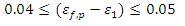
The embedded element technique is adopted to combine two materials together [11]. The cohesive element, a newly proposed technique which can model adhesives, bonded interfaces, gaskets, and rock fracture may be used to simulate interactions between concrete matrix and steel fibres. However, it is impractical to assign the cohesive element to every single steel fibre and in any case, the model developed would probably be too complex to do so. Hence, based on the work by Wille and Naaman, [14], and taking interactions into consideration, some modifications of the constitutive model of steel can be carried out.A bilinear stiffness degradation model is appended to the failure stage of original elastic - perfectly plastic model as shown in the Figure 2. The maximum stress,  is substituted by
  Whereas,
  and
and  can be determined by the sensitivity study carried out later. For this work, the following range of values are recommended, following a series of interim simulations:
 | (5) |
 | (6) |
 | (7) |
 | (8) |
 | Figure 2. Plastic model  for steel material for steel material |
Detailed sensitivity analysis of these parameters can be seen in Section 4.
3. Development of FEA Model
3.1. Generation of Steel Fibres
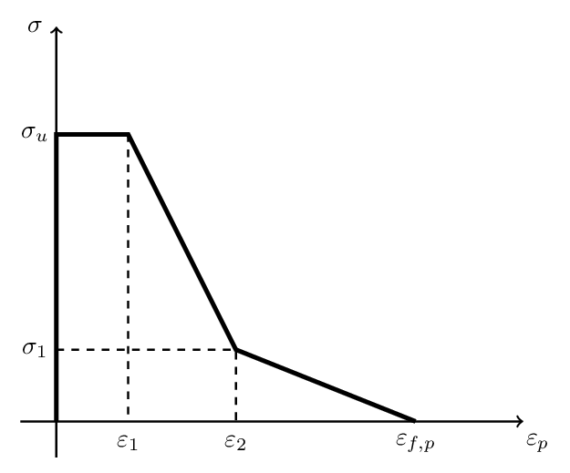
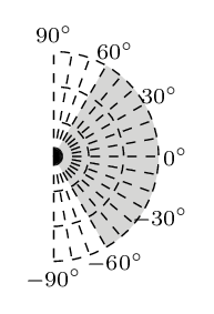
Due to the discrete modelling method employed here the coordinates, hence the position of steel fibres within the mix, can be generated by utilising Monte Carlo methods. This is a technique used to approximate the probability of certain outcomes by running multiple trial runs (simulations), using random variables (sampling) and explore the behaviour of a complex system, like the orientation of steel fibres in a concrete mix. Depending upon the number of uncertainties and the ranges specified for them, a Monte Carlo simulation could involve several thousands of recalculations before it is complete (hence slow convergence can be a downside), producing distributions of possible outcome values [15], [16]. A Monte Carlo simulation can be surprisingly effective in finding solutions to these problems.In this case a set of random numbers can be generated first and then scaled according to different geometric boundaries for different coordinates. The latter can be combined to present the probable orientation (simulation) of steel fibres. Literally, five random numbers are required to define one steel fibre. Details are introduced below.Figure 3 shows the parameters needed to define the orientation of one single fibre in space. A global coordinate system  is established. The origin of the local coordinate system
  can be set to the centre of the fibre. Since the length of steel fibre is known to be 35 mm, five parameters are required to fix one single steel fibre in the global coordinate system: three translational coordinates
  and two rotational coordinates, φ and θ.
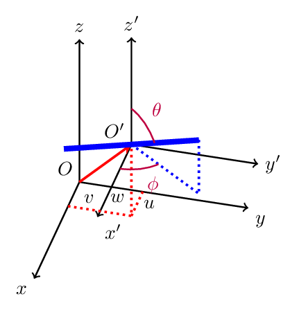 | Figure 3. Coordinate system of a single steel fibre |
3.2. Model Development
The Cracking Model for Concrete is available only in ABAQUS/Explicit. Geometric models can be generated in any CAD system and then can be imported into ABAQUS. For steel fibres, the 2-node linear displacement, T3D2, element can be assigned. For the solid concrete model and the supports, the reduced integration 8-node linear brick with hourglass control, C3D8R, element can be assigned. An Hourglass Effect is essentially a false deformation mode of a Finite Element Mesh. Individual elements are severely deformed, while the overall mesh section is undeformed. This usually happens on hexahedral, 3D solid, reduced integration elements. The displacement controlled load is applied at the RP-1. The final model is illustrated in Figure 4. | Figure 4. The finite element (meshed) model |
4. Analysis and Verification
4.1. An Initial Simulation
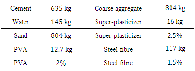
An initial simulation is shown in Figure 5. Experimental data of PVA-PMC 2 and PVA-PMC 3 were brought in from a PhD study by Yougui Lin back in 2012 [10]. The specimens were carried out in accordance with RILEM standards [17]. The dimensions of the beam were 76 mm 100 mm 500 mm  The depth of the notch was 20mm. Table 2 shows mix proportions of the concrete used in the experiment, along with quantities of super-plasticizer, PVA and steel fibre. Details of the mix design can be found in a relevant paper [10].
Table 2. Mix proportions of beam specimen
 |
| |
|
The fibres were 35 mm long, hooked at both ends, with a cross sectional area of 0.27 mm2, an aspect ratio of 60 and a tensile strength of 1050 MPa. Steel fibres are randomly generated in the range of  and
and 
 where
where  and
and  are defined in Figure 3. The parameters of degradation adopted are listed below:
 | (9) |
 | (10) |
 | (11) |
 | (12) |
From Figure 5 it can be said that in general, the simulation trails the mechanical behaviour of the SFRC specimen.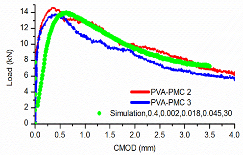 | Figure 5. An initial simulation |
However, Figure 5 encompasses a distinct dive at the beginning (near zero) of the simulation curve. As the load increases linearly to 8 kNit suddenly drops to 2.5 kN, but the corresponding displacement remains negligible. The kinetic energy can be investigated for this.Figure 6 illustrates the kinetic energy and load history for the first second. At a time when the drop takes place, the kinetic energy of the whole system rockets to 0.0243 mJ, roughly ten times of the normal value (approx. 0.002mJ). This is mainly caused by the initial brittle cracking of the matrix. Once the concrete matrix cracks, the strain energy released is partly converted into kinetic energy and then captured again due to the deformation of steel fibres.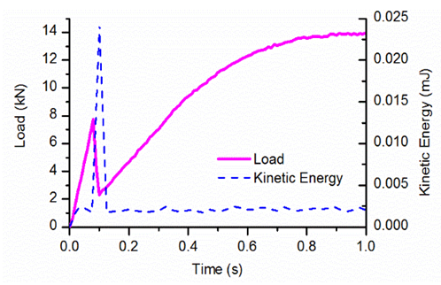 | Figure 6. Kinetic energy and load history |
There is also some discrepancy between the ascending part of the simulated and experimental curves. The initial experimental stiffness is greater while the degradation rate is quicker. Nevertheless, the softening behaviour is clearly detected in the simulation. The maximum load and corresponding crack mouth opening displacement (CMOD) can be predicted well by the simulation, although the predicted CMOD value may be slightly greater than the experimental value. The descending branch of the curve in Figure 5, as customized, can be simulated successfully as long as relative parameters are properly chosen.
4.2. Behavioural Effect of Steel Fibre Orientation
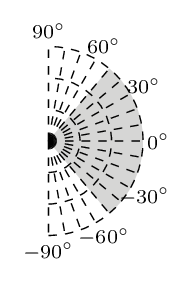
It is widely accepted that the orientation of steel fibres can remarkably influence the mechanical behaviour of SFRC. Hence, as illustrated in the following figures, three different range values of angle  are studied. Please, refer also to Figure 3 for the definition of angle
 | Figure 7. Range values of angle 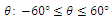 |
 | Figure 8. Range values of angle 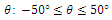 |
 | Figure 9. Range values of angle  |
The simulated results are shown in Figure 10. Parameters in the legend are:  and
and  and
and  successively. It is obvious that angle
  can affect the value of ultimate load. The more horizontal the orientation of the steel fibres, the higher the magnitude of the maximum load achieved. Moreover, the initial rigidity also increases slightly, when the range of angle
  becomes smaller but it also demonstrates that rigidity is not very sensitive to angle
  However, load values at the final stage of the curve seem to overlap (Figure 10), although the peak loads are clearly different. It is reasonable to conclude that models made of different orientation show no distinct behaviour towards the end of the loading procedure because the “fibre bridging effect” is not dominant near the failure stage.
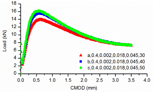 | Figure 10. The effect of orientation  on the load capacity of the specimen on the load capacity of the specimen |
4.3. Behavioural Effect of Steel Fibre Degradation
The stiffness degradation model introduced in the previous chapter is another key factor which can significantly control the response of the beam, especially the tail of the curve. There are four parameters introduced in Subsection 2.2:  and
and  In this section, different combinations of those parameters are tested for the purpose of investigating how the degradation model portrays the response of the beam specimen. Table 3 shows an array of values for these parameters. The steel fibre model illustrated in Figure 7 is used in these analyses.
Table 3. Parameters of nine tested models
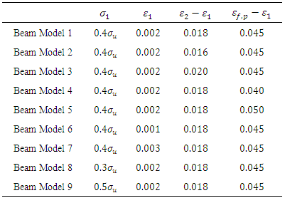 |
| |
|
4.4. Sensitivity Study of  and
and 
Figure 11 shows the results of three models with different  values. The ascending portion of the curve coincides with all three models. The maximum load achieved varies, slightly, with
  The tails are similar. Any (insignificant) differences are due to different peaks. A similar scenario exists in Figure 12 when the variation of load with
  is shown.
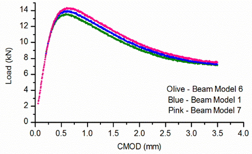 | Figure 11. Variation of load with CMOD for different values of  |
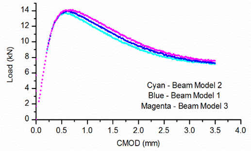 | Figure 12. Variation of load with CMOD for different values of  |
4.5. Sensitivity Study of 
Figure 13 illustrates the effect of parameter  Here, there is no visible difference priorto peak. The tail of the curve begins to deviate at CMOD = 1.3 mm approximately. The final load values are, therefore, slightly different for the three different beam models considered.
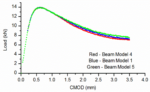 | Figure 13. Variation of load with CMOD for different values of  |
4.6. Sensitivity Study of 
The softening pattern of the mechanical response of the beam model is affected noticeably by the parameter  as shown in Figure 14. However, no difference is shown in the ascending part of the curve but with
  incresing both peak and divergence increase.
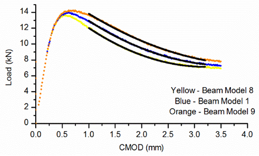 | Figure 14. Variation of load with CMOD for different values of  |
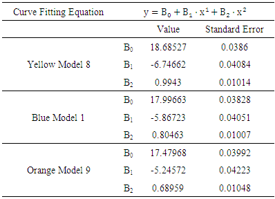
Table 4 shows the curve fitting equation for the softening portion of three simulation results. By studying the equations in the table, it is obvious that the initial resistance descending rate,  increases when
  increases. However, the first derivative of the descending rate, that is the term
  will decrease at the same time.
Table 4. Second order polynomial fitting of the simulation curves
 |
| |
|
5. Conclusions
It is apparent from Section 4 that the numerical model can be used with similar to SFRC material.The main characteristics of the experimental data can be projected well in the simulation. For steel fibre reinforce concrete (SFRC), the fibre plays a vital role in the mechanical response under tensile stress regimes. Slight changes of the constitutive model for steel and/or the distribution of steel fibres can significantly affect the numerical representation and behaviour of the beam specimen.The failure stage of SFRC can be successfully simulated by introducing a steel degradation model into the system.The ascending part of the curve needs more computational effort in order to explain with confidence the jump shown. Adjusting and developing more accurate models to depict the local behaviour is therefore recommended.The descending portion of the curve can be customized by applying different parameters. The solution technique (solver) used can become unstable to some degree, although the problem is not severe.The ascending portion of the experimental curve is stiffer than the simulated one no matter what parameters are adopted but this is not unusual in finite element simulations. The stress softening appears to be smoother in the simulation.The method can only simulate the macro/meso-scale behaviour of SFRC as no fibre bridging law has been introduced in the model. Local stress changes very close to the crack regions cannot be studied. Consequently, crack propagations cannot be tracked numerically. The mechanical behaviour of SFRC structures depends mainly on the orientation of steel fibres in the concrete matrix. The Monte Carlo technique used to generate the steel fibre model in the virtual matrix is, in a way, a game of chance. If the problem can be handled with an analytical or numerical method one should use it. If one has to follow the above method, it is highly recommended to generate the steel fibre model in the simulation more than once.Another key aspect is the bridging law. Although research with regard to pull-out of single fibre has sprung up in recent years, there is still a big gap between the proposed bridging laws and the implementations of them in commercial FEA codes. Exclusive subroutines for this aspect can be designed in the next stage.
ACKNOWLEDGEMENTS
The authors would like to express their gratitude to Dr Yougui Lin, for kindly allowing detailed experimental data from his own Ph.D. thesis to be used in this article.
References
| [1] | Naaman, A. E. (2007) High performance fibre reinforced cement composites: classification and applications. CBM-CI International Workshop. |
| [2] | Rosselló, C., Elices, M. and Guinea, G. V. (2006). Fracture of model concrete: 2. fracture energy and characteristic length. Cement and Concrete Research, 36(7), pp. 1345–1353. |
| [3] | Song, L., Huang, S. M. and Yang, S. C. (2004). Experimental investigation on criterion of three-dimensional mixed-mode fracture for concrete. Cement and Concrete Research, 34 (6), pp. 913–916. |
| [4] | Soroushian, P., Elyamany, H., Tlili, A. and Ostowarid, K. (1998). Mixed-mode fracture properties of concrete reinforced with low volume fractions of steel and polypropylene fibres. Cement and Concrete Composites, 20(1), pp. 67–78. |
| [5] | Abdalla, H. M. and Karihaloo, B. L. (2004), A method for constructing the bilinear tension softening diagram of concrete, corresponding to its true fracture energy. Magazine of Concrete Research, 56(10), pp. 597–604. |
| [6] | Slowik, V., Villmann, B., Bretschneider, N. and Villmann, T. (2006). Computational aspects of inverse analyses for determining softening curves of concrete. Computer Methods in Applied Mechanics and Engineering, 195 (52), pp.7223–7236. |
| [7] | Luccioni, B., Ruano, G., Isla, F., Zerbino, R. and Giaccio, G. (2012). A simple approach to model SFRC. Construction and Building Materials, 37 (0), pp. 111–124. |
| [8] | Radtke, F. K. F., Simone, A. and Sluys, L. J. (2010). A computational model for failure analysis of fibre reinforced concrete with discrete treatment of fibres. Engineering Fracture Mechanics, 77(4), pp. 597–620. |
| [9] | Vanalli, L., Paccola, R. R. and Coda, H. B. (2008). A simple way to introduce fibres into FEM models. Communications in Numerical Methods in Engineering, 24 (7), pp. 585–603. |
| [10] | Lin, Y., Karadelis, J. N. and Xu, Y. (2013). A new mix design method for steel fibre-reinforced, roller compacted and polymer modified bonded concrete overlays. Construction and Building Materials, 48(0), pp. 333–341. |
| [11] | ABAQUS (2010). Abaqus Analysis User’s Manual Volumes 2& 3.DassaultSystèmes. |
| [12] | Wittmann, F., Roelfstra, P., Mihashi, H., Huang, Y. Y., Zhang, X. H. and Nomura, N. (1987). Influence of age of loading, water-cement ratio and rate of loading on fracture energy of concrete. Materials and Structures, 20(2), pp. 103–110. |
| [13] | Cotterell, B. and Mai, Y. W. (1996) Fracture mechanics of cementations materials, 1stedn, Glasgow: Blackie Academic and Professional. |
| [14] | Wille, K. and Naaman, A. E. (2012). Pull-out behaviour of high-strength steel fibres embedded in ultra-high - performance concrete.ACI Materials Journal, 109(4), pp.479–488. |
| [15] | Gentle (2003). Random Number Generation and Monte Carlo Methods. New York: Springer. |
| [16] | Hammersley, J. and Handscomb, D. (1964).Monte Carlo Methods. Methuen’s monographs on applied probability and statistics, Methuen. |
| [17] | RILEM TCS (1985). Determination of the fracture energy of mortar and concrete by means of three-point bend tests on notched beams. Materials and Structures,18 (106), pp.285–290. |

 Abstract
 Reference
 Full-Text PDF
 Full-text HTML