1. Introduction

The safety assessment of dams as costly infrastructures, the failure of which can jeopardize the lives of thousands and play havoc of the downstream land and facilities, is of grave importance. As a result, with many of the already built dams aging and on the other hand the need for new ones to be built, the number of studies conducted on concrete dams has increased significantly. One of the aspects that has always been important in analyzing high concrete structures, and recently has gained well-deserved attention in seismic evaluation of arch dams, is the issue of geometrically nonlinear behavior of these structures considering large displacements when subject to strong ground motions such as MCL earthquakes. This is of great importance not only in theory but also in practical applications. Considering the fact that dams are already built in almost all ideal locations, the engineers are left with no choice but to turn to other sites some of which have high seismicity or are even located on faults. Steno dam (Greece), Shirvan dam (Iran) and Klyde dam (New Zealand) are examples of such cases all of which need geometrically nonlinear analysis for realistic modeling of their behavior[1,2]. Earlier nonlinearstudies carried out on concrete arch dams’ structures can be classified into three groups:

Nonlinear model of joints, including the contraction joints, construction joints and peripheral joints.

Nonlinear model of mass concrete, including tensile cracking models, plastic models and damage mechanics models.

Modeling geometric nonlinearity in the realm of large deformations.

From the first category, studies conducted by Ahmadi et. al [3], Mays et. al[4], Lau et al[5], Hall[6], Ahmadi et. al[7] and Chuhan et. al[8] can be mentioned.

Ahmadi et. al[3] presented a finite elements discrete crack modeling of the dams peripheral and vertical joints. In this study, only the tensile cracks resulting from persistent static loads were taken into consideration. They also developed a method for calculating the failure load which enables the safety analysis of the structures. Lau et al[4] studied the effect of linear and nonlinear behaviors on the magnitude of horizontal tensile stresses in arch dams. The nonlinear model featured three vertical contraction joints.

It was observed that as the result of considering the contractions joints in nonlinear analysis, the tensile stress appearing near the joints in linear analysis is decreased. In this study only three contraction joints of the dam’s ten contraction joints were modeled. This is justified by the results obtained from the study conducted by Fenves et. al[9] indicating that modeling the three joint out of the several joints is enough for reaching the maximum tensile stress and as the number of modeled joints increase, the tensile stress changes from arch to cantilever form.

In another study, Hall et. al[6] developed ADAP-88 software for smeared crack analysis of arch dam. ADAP-88 utilizes a multi-element discretization through the thickness of the dam to model the relative contact in the joints and cracks. Although using inter-element springs models the joints and cracks more realistically, smeared crack model was utilized in this study in favor of less computational cost and better convergence. The software assumes the reservoir water as incompressible. The foundation is mass-less which means there is no energy propagation toward the far end of the model.

Ahmadi et. al[7] presented a discrete crack model of joints, for nonlinear dynamic analysis of concrete arch dam. A joint element model with a tensile-shear behavior was developed in order to analyze the dam-reservoir system more realistically. Chuhan et. al[8] investigated the non- seismic response of Xiaowan and Tujunga arch dams when featuring the contraction joints and reinforcements in joints. The model presented by Fenves et. al[9] (ADAP-88) was utilized for modeling the contraction joints. Factors such as the critical size of the elements, the number of contraction joints and the need for using reinforcement in joints were studied in this research. The reservoir was assumed to be incompressible, the joints behavior was linear-elastic and the foundation was mass less. It was shown that by opening the joint, the nature of the stresses transform from arch to cantilever, as a result the appearance of horizontal cracks in the dam becomes inevitable. In order to reduce the joint opening resulting in this kind of cracks, some steel reinforcement was provided in the model.

From the second category we can refer to researches conducted by Olivier et. al[10], Faria et. al.[11], Lee et. Al [12], Feng et. al[13], Lotfi[14], Watanabe et. al[15] and Mirzabozorg et. al[16,17].

Feng et al. [13] presented a method for stability analysis and crack propagation, based on linear-elastic crack mechanics and 3-D boundary element modeling. In another research by Lotfi et al.[14], a three-dimensional finite elements software was developed for studying the seismic response of arch dams. Non-orthogonal smeared crack approach and elasto-plastic material were implemented in the software modeling. Shahid Rajai dam in Iran was chosen as the case study. It was observed that in the smeared crack model and the elasto-plastic model, the dominant displacement is in the upstream and upward direction. Also it was shown that both smeared crack model and elasto-plastic model overcome defect the large value outputs of stress in linear analysis and give a more realistic prediction of stress distribution in the dam body. Watanabe et al.[15] used a three-dimensional curved surface isoparametric interface element for modeling vertical and peripheral joints. In this study both geometric nonlinearity and material nonlinearity are taken into consideration. For modeling the nonlinear behavior of concrete during loading and failure, a comprehensive elasto-plastic fracture stress-strain relationship, based on elasticity and plasticity theory was used. It was shown that during the earthquake, joint opening results in repeated redistribution of internal forces from arch to cantilever form and vice versa. This phenomenon eventually results in a stable state that is compatible with the real-life behavior of the dam.

In another study by Mirzabozorg[17], a damage mechanics based approach was presented in which cracking occurred non-homogeneously in the elements; meaning that the crack in the elements propagated through Gaussian points. Marrow Point dam was chosen as the case study, for carrying out nonlinear analysis and the dam-reservoir interaction was also taken into account. Foundation was assumed to be rigid, while the reservoir was considered to be compressible and the reservoir bottom to have relative absorption. The proposed approach proved to have acceptable accuracy in predicting the crack propagation rout.

From the third category researches conducted by Chang et al.[18], Youakim et al.[19], Khanloo et al.[20], Swaddiwudhipong et al.[21], Chin et al.[22], Polak et al.[23], Esmond[24], Sathurappan[25], Roca et al.[26], Bathe et al. [27] and Moradloo et al.[28] can be mentioned. Some of these nonlinear geometry studies were carried out on concrete dams and some on other concrete structures. Chang et al.[18] presented the nonlinear geometric seismic analysis of shell structures. Large displacements and large deformations were taken into account and Total Lagrangian approach was used with second Piola-Kirchhoff stress and Green- Lagrange strain. Material was taken as linear elastic and isotropic. Newton-Raphson iterative method accompanied by Newmark method was used for solving the equations. It was observed that in low natural frequencies, the behavior is dramatically affected by the seismic loading, whereas in high natural frequencies this sensitivity becomes less significant.

Nonlinear analysis of tunnels with concrete lining bored into sandy soils was carried out by Youakim et al.[19]. The nonlinear behavior of the problem at hand originated from three sources; nonlinear material behavior of the concrete lining and the soil enclosing it, the effects of large deformations and the nonlinear nature of the sliding between concrete lining and the soil it is in contact with. It was assumed that stress-strain behavior of material is independent from temperature and time. Detail on the utilized formulation can be found in reference[29]. In another study, Khanloo et al.[20] modeled the nonlinear behavior of Tehran’s concrete communication tower. Cracking, crushing and large deformation effects were taken into consideration. Swaddiwudhipong et al.[21] presented a nine-node element for modeling the elasto-plastic large strain response of shell and plate structures using the Updated Lagrangian approach. Chin et al.[22] developed a thin plate element for geometrically nonlinear elastic analysis of thin wall structures. In this study the strains were assumed to be infinitesimal, and Updated Lagrangian approach was implemented.

A methodology for analysis of nonlinear behavior of reinforced concrete shell structures was presented by Polak et al.[23]. Both geometrically nonlinear behavior and material nonlinearity were taken into consideration. Smeared rotating crack method was used for modeling crack propagation. Total Lagrangian approach along with Saint - Venant Kirchhof model was used for accounting for geometrically nonlinear behavior. In order to avoid shear-locking and zero-energy problems, selective integration was used.

Esmond[24] conducted nonlinear geometric, material and time dependent analysis of reinforced concrete shell with edge beams. Geometric nonlinearity of the structure was assumed to stem from infinitesimal displacements and rotations. Concrete model was based on nonlinear elasticity with assumption of orthotropic material. Material nonlinearities include tensile cracking, tension stiffening between cracks, the nonlinear response of concrete in compression, and the yielding of the reinforcement are considered. Total Lagrangian approach along with Saint-Venant Kirchhof model was used for accounting for geometrically nonlinear behavior.

Sathurappan et al.[25] performed the nonlinear analysis of reinforced and pre-stressed reinforced concrete slabs. Geometric nonlinearities and material nonlinearities were both considered in the study. Material nonlinearity of concrete was modeled by assuming plasticity in compression and cracking in tension. Total Lagrangian approach along with Saint-Venant Kirchhof model was used for accounting for geometrically nonlinear behavior.

Numerical treatment of pre-stressing tendons in the analysis of reinforced concrete structures nonlinear behavior was investigated by Roca et al.[26]. Updated Lagrangian approach along with hypo-elastic model ofDarwinandPecknold was used for accounting for geometrically nonlinear behavior. Concrete material behavior in tension is assumed to be elasto-brittle.

By presenting the characteristics of concrete used in ADINA software and some of its usages, Bathe et al.[27], suggested utilization of second Piola-Kirchhoff stress and Green-Lagrange strain (Saint-Venant Kirchhof model) for modeling large displacements in concrete structures.

Moradloo et al.[28] used the Saint-Venant Kirchhof behavior model for large deformations to analyze the behavior of concrete arch dams during seismic excitation. The foundation was assumed to be rigid and the water-structure interaction was modeled by using the concept of added mass. For demonstrating the importance of large deformation effects, Marrow Point dam was analyzed using a nonlinear hyper-elastic model. Other sources nonlinearity such as joint opening and concrete material nonlinearity were ignored. Considering the characteristics of concrete such as not admitting large strains, Lagrangian approach along with Saint-Venant Kirchhof model was chosen for accounting for geometrically nonlinear behavior of non-reinforced concrete. It was shown that considering the effects of large deformations, can increase the displacement response of the dam crest by 11 percent in strong ground motions. Considering the characteristics of concrete arch dams it is expected that this increase in response become even more significant if the following features are also taken into account in the analysis:

Water penetration effect in joints and cracks

Vertical and peripheral joints opening and sliding effects

As it can be seen, in spite of the fact that several studies involving geometric nonlinear analysis of shells and plates structures have been carried out earlier[2], geometric nonlinear behavior of concrete dam has been given little attention in all the earlier researches.

In the present study, co-rotational formulation for geometrically nonlinear analysis of concrete arch dams is presented. Using the presented formulation, nonlinear dynamic analysis of Dez arch dam under Manjil MCL earthquake is conducted to show large deformation effects. Foundation is assumed to be a mass-less flexible medium and Fluid- structure interaction is modeled including water compressibility and reservoir bottom absorption. Other source of nonlinearity in the analysis is joint opening. Concrete material nonlinearity is ignored. The penetration of water in opening joint during the earthquake is also considered and the significance of nonlinear geometry effects when accompanied by hydrodynamic pressure in joints is investigated.

2. Basic Concepts of Geometric Nonlinearity and Methodology Layout

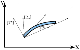
Structural nonlinearities may be caused by three main reasons, (a) material nonlinearities, (b) changing status, and (c) geometric nonlinearities. The key difference between the problems with geometric nonlinearity and other kinds of nonlinearity lies in the kinematics. The problems of geometric nonlinearity are usually dealt with, by tracing the geometrical changes in the structure and its elements with reference to a reference state, in an incremental manner. The increasing changes in the geometry of the structure due to proportionally growing applied forces may ultimately lead to elastic instability of the structure and its consequent failure. In this paper the effects of geometric nonlinearities on the seismic response of concrete arch dams is investigated.

Generally there are two main distinct types of instability scenarios possible in geometrically nonlinear problems. These two kinds of instability behaviors depend closely on the concepts of limit point and bifurcation point on the load-displacement or equilibrium path of the structure. Description on these two mentioned types of structural instability behavior can be found in a number of papers published so far [e.g. 30,31] and hence is not elaborated on further, here.

2.1. Large Deformation Model

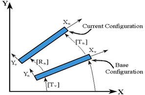
A large deformation model consists of three main parts: A) Mesh Description and Governing equation, B) Constitutive Relation and C) Equation Linearization and solution algorithm.

In a nonlinear analysis, the equilibrium of the body considered must be established in the current (deformed) configuration. Also it is necessary to employ an incremental formulation to confidentially describe the loading and the motion of the body. Also a suitable constitutive model is needed.

In recent years, theoretical formulations and computational methods for dealing with geometric nonlinearities in the structures have been the focus of much attention[32-33]. In general, four approaches exist in kinematic modeling of geometrically nonlinear problems: Spatial or Eulerian Description, Material or Lagrangian, Arbitrary Eulerian- Lagrangian Description (AEL) and Co-rotational Description [28]. Each of these formulations can be useful for certain constitutive equation or loading conditions by decreasing the number of required transformations.

In Eulerian approach the fact that the material and mesh movements are independent, poses difficulties in dealing with solid media when implementing the boundary conditions [28]. As a result, it is commonly used in fluid dynamics. In the Eulerian description large distortions in the motion of continuum can be dealt with more easily than Lagrangian approach, but generally at the expense of precise interface definition and resolution of flow details[34].

ALE approach overcomes the shortcomings of purely Lagrangian and purely Eulerian descriptions. In the ALE description, nodes on boundary of initial mesh are fixed during deformation and nodes in the middle move such that element distortion will be minimized. In fact, the nodes of the computational mesh can be dragged along with the material particles as in Lagrangian approach, be held fixed similar to Eulerian manner, or be moved in some arbitrarily specified way to provide a continuous rezoning capability. Indeed by offering this freedom in moving the computational mesh, the ALE description retains the advantages of above- mentioned approaches while avoiding their disadvantages. Meaning that greater distortions of the continuum can be handled than that permitted in a purely Lagrangian method and with more resolution that what is allowed by a purely Eulerian approach.[28,34]

The Lagrangian description is one of the most popular descriptions developed so far. In the Lagrangian approach a Cartesian coordinate system is employed to trace the structural deformation during loading history[28] that is, each material particle is followed by an individual node of the computational mesh associated with it, allowing easy tracking of free surfaces and boundaries between different materials. Also materials with history dependent constitutive relations are treated easily with Lagrangian approach [34] (arbitrary Lag-Eul methods). Depending on the way the deformations are described, the Lagrangian approach yields three main subgroups which are applicable in geometrically nonlinear analysis.

Total Lagrangian Description (TLD) is the first type, in which the element’s original frame of reference is used to assess the deformations of the element and all the following element deformations are attributed to the same frame of reference and therefore the displacement variables involved in the derivation of element stiffness matrices in the former framework are the total instead of the incremental quantities [35]. In the total Lagrangian formulation the integrals in the weak form are carried out over the initial (reverence) configuration and derivatives are taken with respect to the material coordinates[28]. The ease of implementation is an advantage to this method. However, considering the fact that this method is unable to tell apart the rigid body motion of the element from its local deformation, this defect results in incorrect description of the equilibrium path, unless the rotations and deflections in the problem are small[32].

Updated Lagrangian Description (ULD) is the second type. In this method the current configuration is taken as the reference frame for the following step and by doing so the inability of TLD in distinguishing the rigid body motions from local deformation is overcome. In the update Lagrangian formulation, the derivatives are obtained with respect to the spatial coordinates; the weak form involves integrals over the deformed (or current) configuration. This method yields a more precise description of the displacement field of elements and the structure. In UL formulation there is no need to calculate initial stiffness in each iteration. Also in using UL formulation the artificial straining does not occur [35]. However, the calculation of the local element deformation during each stage of loading proves to be laborious. In addition, when it comes to developing a consistent set of equilibrium equations for incremental analysis, the transformation of the tangent stiffness matrix from local to global axes calls for a great deal of matrix operations [36]. As a result this type of description of displacement has not become much appealing in practical structural applications unless, the problem is of elastic nature and involves very large defections.

Partially Updated Lagrangian Description (PULD), as the third derivation of the Lagrangian approach, utilizes the idea of the rigid-convected coordinates’ method as in ULD formulation. In this approach the coordinates of each element is are updated only once at the start of each loadstep then the numerical operations within each loadstep are then carried out as in TLD approach. This type of formulation has both of the advantages of the simplicity in TLD formulation and the accuracy in ULD formulation at the same time. Interested reader is referred to[37-39] for more detail on this type of formulation.

In concrete dam analyses, since small strain, element large distortion is not occurs and if initial finite element mesh well designed there is no anxiety about distortion and following precise reduction in results. Geometric nonlinear of arch concrete dam is a nonlinear problem with large displacement and small strain. With respect to stage construction of arch concrete dam and concrete purities itself it expected that under severe earthquake loading, dam monoliths experienced large slip and large deformation caused by joint opening and failure with amount of crushing and plastic deformations.

The description utilized in the current study is the co-rotational (CR) approach. This approach is identical to PULD except for the fact that in the former, the element coordinate systems are rotating during the time steps. In Co-rotational approach initial configuration consists of two parts, stresses and strain calculated from rotated configuration and rigid body motion deduced from initial configuration. In this method the FEM equations of each element are attributed to two systems (as shown in figure 1):

A fixed or base configuration C_B as in TLD.

A co-rotated configuration that is dragged along with the element an in fact is a rigid body motion of C_B. This is fairly similar to ULD.

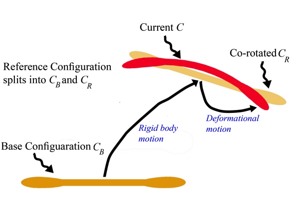Figure 1. The CR kinematic description; “Current configuration” means any one assumed by the body or element during the analysis process. It is not necessarily an equilibrium configuration[35]

The main idea behind CR description is the separation of the reference configuration into two other configurations. One of them is the base configuration that remains fixed during the analysis and acts as a fixed reference configuration CB. The coordinate system corresponding to this reference configuration is the same for the whole structure; the reference configuration in a Co-rotational formulation continuously translates and rotates with the element, but does not deform with it. The other one is the co-rotated configuration CR which changes from one element to the other. For each element its CR configuration is obtained in the form the rigid body motion of the base element. The coordinate system that is connected to this configuration is Cartesian and moves simultaneously with the element like a “shadow”. Element deformations are calculated with respect to this configuration. The equilibrium equation in the Co-rotational approach is formulated from the principle of stationary potential energy, which yields the element secant stiffness matrix[35,40].

One of the advantages of co-rotational formulation to total and updated Lagrangian approaches is that because of the fact that the rigid body motion of the element is separated from its deformation, the degrees of freedom that enter the elements formulation are decreased by the number of rigid body modes. As the result, the effects of rigid body motion do not appear in the tangent stiffness matrix (natural tangent stiffness matrix). To account for the rigid body rotations of the element, the element’s tangent stiffness matrix is complemented by a stability matrix[35].

Another advantage of co-rotational approach is that the integrations on the volume of the element are preformed over the reference configuration which is unreformed during the analysis, whereas in Updated Lagrangian approach, the formulation dictates that the integration be performed over the complicated deformed shape of the element at the last configuration computed so far[41]. In many studies employing the Updated Lagrangian approach[40,42-46] it is assumed that the elements remain straight during loading, but Lip H. et al.[47] showed that this assumption in UL approach can result in significant inaccuracies in framed structures the members of which undergo considerable bowing deformations and co-rotational framework yields better results. Moreover, the issue regarding the ‘assumption’ of a straight configuration is irrelevant in the Co-rotational formulation, since the reference configuration is the undeformed configuration of the (straight) beam element.

In the corotational approach, the nonlinear stress and strain fields are calculated as viewed by a corotational local observer moving with the element, then the obtained description of stress and strain are transferred to a fixed global coordinate system directly by employing the change-in-the- observer algebra. A very important advantage this procedure provides is that the recovered nonlinear structural models implicitly meet objectivity criteria (meaning that they are geometrically exact)[48]. As a result engineering stress and strain measures can be used in the Co-rotational method.

2.2. Implementation of Corotational Approach

The strain-displacement nonlinearity in the CR approach is described as[49],

(1)

where:

[Bv]= usual small strain-displacement relationship in the original element coordinate system

[Tn]= orthogonal transformation that relates the original element coordinates to the convected (or rotated) element coordinates

The difference between the rotated element coordinate system and the original element coordinate system is the result of rigid body rotation. Therefore in order to calculate [Tn], we need to separate the rigid body rotation from the total deformation {un}. Utilizing the polar decomposition theorem:

(2)

where:

[R] = rotation matrix ([R]^T[R] = [I])

[U] = right stretch (shape change) matrix

The element tangent stiffness matrix is obtained from (1) as,

(3)

The element restoring force vector is,

(4)

In the above equation, the elastic strain is obtained from,

(5)

The vector describes the element deformation, which causes the strain to appear. For each element the large rotation approach can be described in three steps:

1. The element updated transformation matrix [Tn] is calculated

2. The deformational displacement is obtained from the total displacement {u_n} in order to calculate the restoring force and the stresses.

3. Node rotations are updated according to the computed rotational increments in.

Effective implementation of the three steps above requires the concept of a rotational pseudo-vector[].

2.2.1. Element Transformation

As mentioned earlier, the updated transformation matrix [T_n] transforms the current element coordinate frame to the global Cartesian coordinate system (see Figure 2).

Figure 2. Element Transformation Definitions[49]

The updated transformation matrix [T_n] can be related to the rotation of the element coordinate system [R_n] and the original transformation matrix [T_v] by,

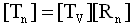(6)

2.2.2. Deformational Displacement

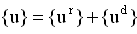
The displacement an element undergoes can be decomposed into a rigid body translation, a rigid body motion, and a components that causes the strain,

(7)

where:

{u^r} = rigid body motion

{u^d} = deformational displacements which cause strains which includes both translational and rotational DOF.

The translational component of the deformational displacement can be obtained from the displacement field by

(8)

where:

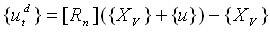
= translational component of the deformational displacement

[R_n] = current element rotation matrix

{x_v} = Original element coordinates in the global coordinate system

{u} = Element displacement vector in global coordinates

{u^d} is in the global coordinate system.

The rotational components of DOFs are calculated by subtracting the nodal rotations {u} from the element rotation {u^r}. This operation is performed as follows for each node (utilizing the pseudo-vectors):

1. A transformation matrix from the nodal pseudo-vector {θⁿ} is calculated, yielding [T_n].

2. The relative rotation [T^d] between [R_n] and [T_n] is computed:

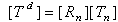(9)

This relative rotation consists of the rotational deformations of that node as shown in Figure 3.

Figure 3. Definition of Deformational Rotations[49]

2.2.3. Updating Rotations

After obtaining the transformation [T] and deformational displacements {u^d}, the element matrices and restoring force can be calculated from equations (3) and (4), respectively. A displacement increment {Δu} results from the solution of the system of equations. The rotational components of {Δu} are used to update the nodal rotations at the element level. The global rotations are updated simply by adding to the previous rotation in {u_n-1} and by the pseudo-vector approach.

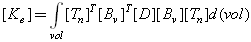
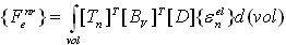
2.2.4. Consistent Tangent Stiffness Matrix and Finite Rotation

The use of consistent tangent stiffness in a nonlinear analysis can speed up the convergence trend to a quadratic rate of convergence. A consistent tangent stiffness matrix is derived from the discretized finite element equilibrium equations without the introduction of various approximations.

The process of deriving of the consistent tangent stiffness matrix used for the corotational approach is outlined below [49,50].

For each element, the nonlinear static finite element equations solved are defined as:

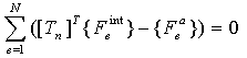(10)

where:

N = number of all elements

= element internal force vector in the element coordinate system,

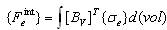(11)

[T_n]^T = transform matrix, transferring the local internal force vector into the global coordinate system

= Applied load vector at the element level in the global coordinate system

Now we derive the consistent tangent matrix at the element level without introducing an approximation. The consistent tangent matrix is obtained by differentiating equation (10) with respect to displacement variables {u_e}:

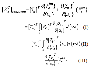(12)

It can be seen that Part I is the main tangent matrix (equation (3)) and Part II is the stress stiffening matrix. Part III is another part of the stress stiffening matrix[49,51] which is usually negligible. Numerical solution of nonlinear equations has been subject to ample research and various methods have been proposed to tackle this kind of problems, one of the oldest and most reliable of which is the Newton-Raphson method[49]. In this method the load is divided into a number of load increments. The load increments are then applied through a number of loadsteps. In the present study full Newton-Raphson study procedure was employed which updates the stiffness matrix at each equilibrium iteration.

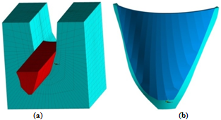Figure 4. (a) Dam-Reservoir-Foundation finite element model and (b) Dam body and the concrete saddle

3. Numerical Model of a Typical High Arch Dam

Dez double curvature arch dam in Iran is selected as the case study. Crest length is 240m and thickness at the crest level is 4.5m (Figure 4). Finite element idealization prepared for the dam, foundation rock and reservoir is shown in Figure 4a, which consists of 792 solid elements for modeling the dam body and its concrete saddle, 3770 solid elements for simulation of the foundation rock and 3660 fluid elements in the reservoir domain. In addition, 956 node-to-node contact elements are used to model vertical and peripheral joints of the dam. Figure 5 shows the surfaces on which the contact elements are located.

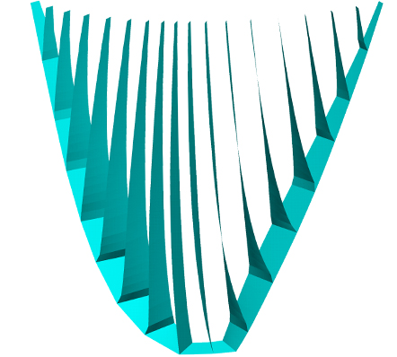Figure 5. Vertical and peripheral joints in DEZ dam

3.1. Basic Mechanical and Strength Parameters

Water is assumed to be compressible with density of 1000kg/m³. The speed of sound in water is 1440m/s and the wave reflection coefficient at the boundaries of the reservoir with the abutments and at its bottom is taken to be 0.8, conservatively. A viscous boundary at the far end of the reservoir dissipates the waves reaching this boundary and prevents them from being reflected back into the reservoir. Having neglected the sloshing effects, we have imposed zero pressure boundary condition for reservoir free surface. This assumption is acceptable for high dams[52,53]. Table 1 shows the material properties for the mass concrete and the foundation of the model[54,55]

Table 1. The material properties for the mass concrete and the foundation of the model Static properties Dynamic properties Mass Concrete Isotropic Elasticity 40GPa 46GPa Poisson’s Ratio 0.2 0.14 Density 2400kg/m3 2400kg/m3 Thermal Expansion Coefficient 6×10-6/℃ 6×10-6/℃ Compressive Strength 35MPa 36.6MPa Uniaxial Tensile Strength 3.4MPa 5.1MPa Isotropic Elasticity- Saturated 13GPa 13GPa Foundation Isotropic Elasticity- Unsaturated 15GPa 15GPa Poisson’s Ratio 0.25 0.25

3.2. Loading

The loads applied to the model in chronological order are, self-weight of the dam body (during 10 stages of construction and sequential joint grouting), hydrostatic pressure (considering gradual impoundment), thermal loading (summer condition, obtained from transient thermal analysis of the dam including solar radiation phenomenon [55]) and finally the seismic excitation. The coupled nonlinear dam-reservoir-foundation system problem is solved employing the β-Newmark time-integration method. For dynamic analysis, the system is excited in maximum credible level using Manjil earthquake scaled based on response spectrum of the dam site. Table 2 presents the characteristics of Manjil ground motion.

Table 2. The characteristics of MANJIL ground motion Ground motion MANJIL-June 21, 1990 Component (φ°) Transverse Longitudinal Vertical PGA (g) 0.310g 0.387g 0.260 g

For obtaining the strong motion duration of the earthquake, Arias intensity on Husid diagram is utilized and then time interval between 5% and 95% of Arias intensity based on Trifunac and Brady theory is selected[56]. The strong motion duration is determined to be 30s for the selected earthquake. Considering that arch dams response to earthquake is most critical when they are excited in upstream-downstream direction, the major direction of the ground motion is applied to the system in upstream-downstream direction (in the provided model, Y axis)[57]. All three components of the seismic ground motion are applied to the dam- foundation-reservoir system simultaneously. Structural damping is assumed to be 10% of critical damping, and mass and stiffness proportional damping coefficients αM and βK are obtained using Rayleigh damping method. It is noteworthy that all the analysis results presented in this paper include the dam response up to the 8th second of the seismic excitation. The results for the rest of the ground motion duration were excluded since the dam did not show any significant change in its behavior in the rest of the analyses.

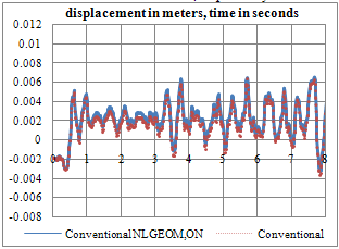
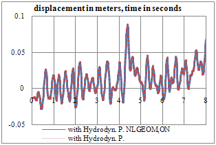
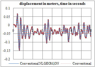Figure 6. Upstream-Downstream displacement time-history of crown cantilever at crest level (Conventional analysis)

4. Results and Discussion

4.1. Crest Displacement

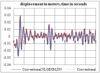
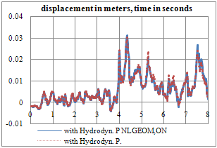
Figures 6 to 8 compare the crest displacement in the three principal directions for the two cases of with and without geometric nonlinearity. In addition, Table 3 represents briefly the extreme values resulted from the conducted analyses. As can be seen, when hydrodynamic pressure is applied in the open joints, geometric nonlinearity can lead to about 5% increase in upstream-downstream extreme displacement. The corresponding values for transvers and vertical directions are 7.5% and 1.4%, respectively.

Figure 7. Transverse displacement time-history of crown cantilever at crest level (Conventional analysis)

Figure 8. Vertical displacement time-history of crown cantilever at crest level (Conventional analysis)

Figures 9 to 11 show the time-history of the crest at the crown cantilever when there is no water penetration into the open joints. Also, the results are presented briefly in Table 3. It is found that the geometric nonlinearity has little effect on the response so that in upstream-downstream direction, the change in extreme values is less than 0.1%, which is negligible.

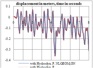Figure 9. Upstream-Downstream displacement time-history of crown cantilever at crest level (with Hydrodynamic pore-pressure in joints)

Figure 10. Transverse displacement time-history of crown cantilever at crest level (with Hydrodynamic pore-pressure in joints)

Figure 11. Vertical displacement time-history of crown cantilever at crest level (with Hydrodynamic pore-pressure in joints)

Table 3. Comparison of displacement results With hydrodynamic pore pressure in joints Without hydrodynamic pore-pressure in joints Conventional With G.N.L.E Conventional With G.N.L.E Max min min max max min min max Transverse Value (m) 0.030132 -0.00377 -0.00405 0.031023 0.009739 -0.00595 -0.0056 0.00982 time (s) 4.34 3.62 3.62 4.34 9.06 8.78 8.78 9.06 Change in percent 7.427% -5.882% 2.956% 0.831% Upstream -Downstream Value (m) 0.070307 -0.35836 -0.35834 0.073739 0.067721 -0.14765 -0.14768 0.067665 time (s) 0.42 4.4 4.4 3.64 0.42 0.62 0.62 0.42 Change in percent -0.005% -0.020% 4.881% -0.082% Vertical Value (m) 0.088217 -0.02781 -0.02819 0.086866 0.029362 -0.02646 -0.0277 0.028224 time (s) 4.4 0.44 0.44 4.4 0.62 0.42 0.42 0.62 Change in percent 1.366% 4.686% -1.531% -3.875% With G.N.L.E= with geometric nonlinearity effects Conventional= without geometric nonlinearity effects

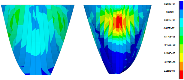Figure 12. Non-coincident push of 1st principle stress in analysis with hydrodynamic pressure in joints, by loadstep 400 (second 8)

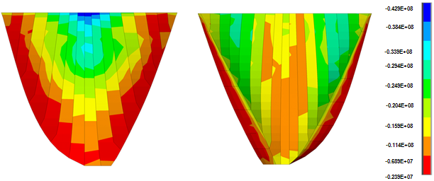
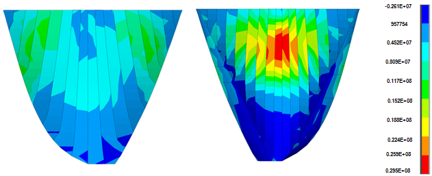
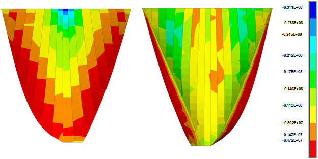
4.2. Stress Distribution

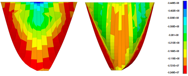
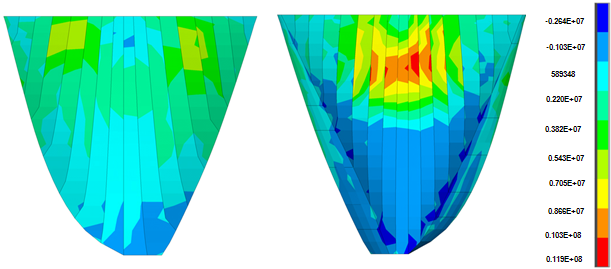
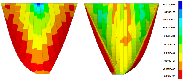
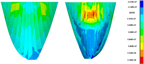
Figures 12 and 13 show the non-coincident envelope of the first and third principal stresses when water can penetrate into open joints and Figure 14 and 15 show the corresponding envelopes when geometric nonlinearity is accounted for. Table 4 represents briefly the extreme values of the principal stresses for various cases. Based on the shown envelopes and the table, the effect of geometric nonlinearity is negligible so that there is not any change in maximum tensile stress and the maximum compressive stress increases just about 4.7%.

Figures 16 and 17 show the envelopes pertinent to the non-coincident principal stresses when there is no water penetration in open joint and Figures 18 and 19 represent the corresponding stress envelopes when geometric nonlinearity is taken into consideration in the conducted analysis and finally, Table 4 represents the results briefly. As expected, when water penetration is not permitted, the effect of geometric nonlinearity is almost imperceptible.

Figure 13. Non-coincident push of 3rd principle stress in analysis with hydrodynamic pressure in joints, at loadstep 400 (second 8)

Figure 14. Non-coincident push of 1st principle stress in analysis with hydrodynamic pressure in joints, by loadstep 400 (second 8) with geometric nonlinearity effects

Figure 15. Non-coincident push of 3rd principle stress in analysis with hydrodynamic pressure in joints, at loadstep 400 (second 8) with geometric nonlinearity effects

Figure 16. Non-coincident push of 1st principle stress in conventional analysis, by loadstep 400 (second 8)

Figure 17. Non-coincident push of 3rd principle stress in conventional analysis, at loadstep 400 (second 8)

Figure 18. Non-coincident push of 1st principle stress in conventional analysis, by loadstep 400 (second 8) with geometric nonlinearity effects

Figure 19. Non-coincident push of 3rd principle stress in conventional analysis, at loadstep 400 (second 8) with geometric nonlinearity effects

Table 4. Comparison of stress results With hydrodynamic pore pressure in joints Without hydrodynamic pore-pressure in joints Conventional With G.N.L.E Conventional With G.N.L.E S1 S3 S3 S1 S1 S3 S3 S1 Exterimum Value up to second 8 0.295E+08 -0.429E+08 -0.449E+08 0.295E+08 0.119E+08 -0.311E+08 -0.311E+08 0.120E+08 Change in percent 4.662% 0% 0% 0.840% With G.N.L.E= with geometric nonlinearity effects Conventional= without geometric nonlinearity effects S1= first principle stress S3= third principle stress

Figure 20. Non-coincident push of joint openings (Gap on the left & Sliding on the right) in analysis with hydrodynamic pressure in joints, by loadstep 400 (second 8)

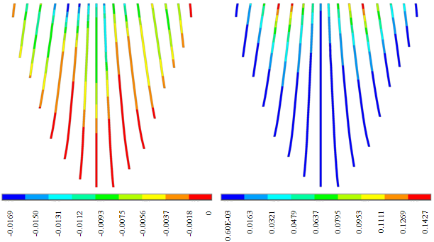
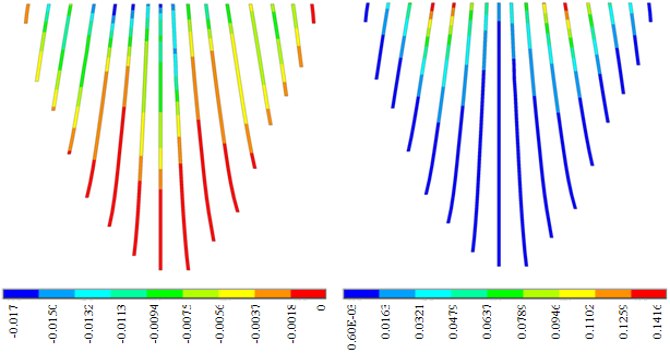
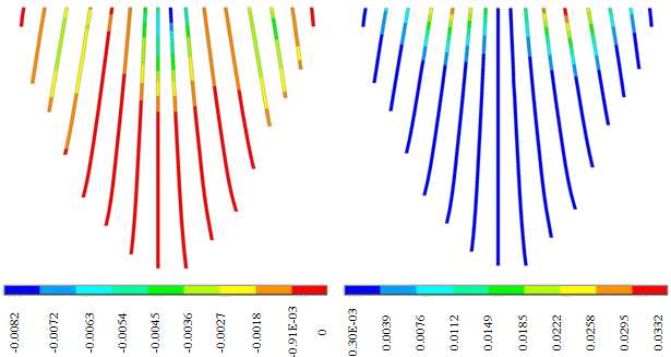
4.3. Joint Opening/Sliding

Figure 20 shows the non-coincident envelope of the joints’ opening and sliding when water can penetrate into open joints and Figure 21 shows the corresponding envelopes when geometric nonlinearity is accounted for. Table 5 briefly represents the extreme values of the joint responses for various cases. Based on the shown envelopes and the table, it can be seen that when hydrodynamic pressure is applied in the open joints, the effect of geometric nonlinearity on joint opening is negligible.

Figures 22 shows the envelope of the joints’ opening and sliding when there is no water penetration in open joints and Figure 23 represents the corresponding opening envelopes when geometric nonlinearity is taken into consideration in the conducted analysis and finally, Table 5 summarizes the results briefly. When water penetration is not permitted, the joints’ sliding is decreased by 3.6% due to geometric nonlinearity and there is no noticeable change in joint opening.

Figure 21. Non-coincident push of joint openings (Gap on the left & Sliding on the right) in analysis with hydrodynamic pressure in joints, by loadstep 400

Figure 22. Non-coincident push of joint openings (Gap on the left & Sliding on the right) in conventional analysis, at loadstep 400 (second 8)

Table 5. Comparison of joint opening results With hydrodynamic pore pressure in joints Without hydrodynamic pore-pressure in joints Conventional With G.N.L.E Conventional With G.N.L.E Gap Sliding Sliding Gap Gap Sliding Sliding Gap Exterimum Value up to second 8 -0.0169 0.1427 0.1416 -0.017 -0.0082 0.0332 0.032 -0.0079 Change in percent -0.770% -3.614% 0.591% -0.0079% With G.N.L.E= with geometric nonlinearity effects Conventional= without geometric nonlinearity effects S1= first principle stress S3= third principle stress

4.4. Discussion

In the previous sections, the results obtained from four nonlinear analyses considering construction joints effects were presented. The analyses were different from the point of considering the effects of geometric nonlinearity including/excluding water penetration into open joints. Based on the presented results, geometric nonlinearity effect on the structural behavior is magnified when water penetration is permitted. However, this effect is negligible. The insignificant effect of geometric nonlinearity on the dam behavior is justifiable by the fact that the nonlinear material behavior of mass concrete was excluded in the present study. Considering the fact that one of the main sources of nonlinear behavior in MCL condition is material nonlinearity in tensile and compressive states in mass concrete and taking it into account, increases the displacement response of the dam, it is predicted that geometric nonlinearity will have a more noticeable effect on the dam response. This case is the subject of the future study by the authors.

5. Conclusions

In the present paper the effects of nonlinear geometry on the seismic response of a real-life high arch dam model was investigated. Co-rotational approach was utilized for formulating the large-deformation phenomenon. The behavior of mass concrete was assumed to be linear while all of the construction and peripheral joints were modeled according to as-built construction details. The reservoir water was assumed to be compressible and the foundation rock was modeled as a mass-less medium. It was observed that when water penetration in opening joints of the dam is permitted during the excitation, the response of the dam increases, nevertheless this increase in the dam response is insignificant. According to authors experience and engineering judgment, it is predicted that considering the material nonlinearity will magnify the effects of geometric nonlinearity.