S. P. Dashuk, V. F. Borisov
A.P. Alexandrov Research Institute of Technology (NITI), 188540, Sosnovy Bor, Leningrad region, Russia
Correspondence to: S. P. Dashuk, A.P. Alexandrov Research Institute of Technology (NITI), 188540, Sosnovy Bor, Leningrad region, Russia.
| Email: |  |
Copyright © 2014 Scientific & Academic Publishing. All Rights Reserved.
Abstract
This paper describes the design concepts of digital-to-analog simulators of nuclear reactor reactivity and gives information pattern about power signal which corresponds to fixed value of reactivity. The main design concept for digital-to-analog simulator is decadic partition of power signal level with normalization of decades to the specified number which corresponds to number of bits of digital-to-analog converter (DAC) and storing of the duplicated information concerning the power signal. This paper proposes the design of simulator based on 12-bit DAC. The simulator has ≤1% relative error for reactivity value corresponding to output signal of DAC-simulator within three decades of power signal variation.
Keywords:
Nuclear Reactor, Power Signal, Reactivity, Digital-to-Analog Simulator
Cite this paper: S. P. Dashuk, V. F. Borisov, Simulator of Reactor Kinetics, International Journal of Instrumentation Science, Vol. 3 No. 1, 2014, pp. 1-7. doi: 10.5923/j.instrument.20140301.01.
1. Introduction
For reactor monitoring, special-purpose calculation instruments called reactivity meters are widely used [1, 2]. Functional principle of reactivity meter is based on the solution of reversed equation of reactor kinetics with input signal proportional to neutron flux [1].Periodic calibrations and function tests of the reactivity meters should be performed in order to support reliable operation of reactor control system. For this purpose specialized instruments, simulators of reactor kinetics, are used. These simulators can also be used for adjustment of reactivity meters in factory and for testing of instruments of the reactor control and safety system.The simulator output signal models variation of neutron flux (reactor power) at constant value of reactivity, the variation corresponding to solution of the known set of neutron kinetics equation [3]: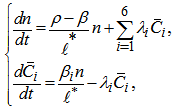 | (1) |
where n is the neutron density; βi, λi, are the characteristics of the i-th delayed neutron group; β is the fraction of delayed neutrons; ℓ* is the prompt neutron lifetime;  is the concentration of the i-th group delayed neutron precursors; ρis the value of reactivity.Ideally the output signal of simulator should correspond strictly to solution of differential equation system (1) with respect to n(t) at constant value of reactivity which should be set in the simulator, i.e. output voltage U(t) or current I(t) versus time is given by:
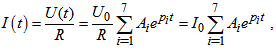 | (2) |
where I0 is the initial current at the simulator outlet; U0 is the initial voltage at the simulator outlet; R is the resistance of current-forming resistor; pi are the roots of characteristic equation resulted from (1); Ai are the coefficients whose values depend on the reactivity value set in the simulator.In other words, ideally the output signal of the simulator should be formed such that the value calculated from this signal is identical to the set value. In reality this signal can have some deviations from the ideal one for a number of reasons. Consequently, there will be an error in the calculated reactivity value. For the sake of simplicity, this error is hereinafter referred to as the reactivity modeling error.Until quite recently, a traditional approach to developing reactivity simulators has been to use analog simulation of reactor kinetics equations [4] where the connection between model and reactor parameters is determined by the following equations: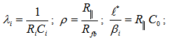
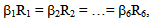 where ρ, β is the set value of reactivity; R||, Ω is the resistance equal to parallel connection of Ri; Rfb, Ri, Ω are the corresponding values of resistance; Ci, C0, F are the corresponding values of capacitors. Figure 1 shows an electrical model of reactor kinetics, which corresponds to (2). The parameters of this model can be calculated using physical characteristics λi, ℓ* and αi=βi/β. A1 is the measuring amplifie; A2, A3 are the scaling amplifiers; C0 is the capacity simulating prompt-neutrons lifetime; RiCi are the six RC circuits, simulating six groups of delayed neutrons; VS is the voltage source for initial condition adjustment; Rfb is the set of feedback resistors, which determine the set reactivity; RT is the voltage-current resistive transducer; S1 is the switch of voltage source; S2 is the switch of modeling start; S3 is the positive\negative reactivity switch.
 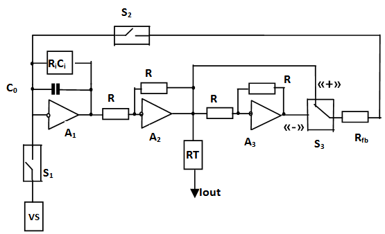 | Figure 1. Electrical model of reactor kinetics (analog simulator of reactivity) |
The main limitation of the analog circuit is slow changeover between simulation modes because long-time constants are needed for recovery of initial conditions in RC-circuits. In practice this leads to considerable time losses during preparation of the simulator for operation, because after each simulation change 5-10 minutes delay is required before the initial conditions can be set. Moreover, the parameters of RC-circuits of the analog simulator should be chosen taking into account a specific fuel composition or specific type of reactor. Therefore, modification of the electric circuit and its parameters is required to perform calibration of reactivity meters used for measurements in reactors with different fuel compositions or different type reactors. Finally, error of reactivity modeling sharply increases in analog simulators during formation of the output signal which corresponds to negative reactivity after a few decades of the output signal change («far-field error»), because in this case the desired signal value of the measuring amplifier decreases by a few decades and approaches becomes commensurable to the simulator noise.
2. Digital-to-analog Simulator of Reactivity
A good alternative to analog simulator is a reactivity simulator based on digital-to-analog converter – the function which is widely used in different technical fields [5-7]. In D/A reactivity simulator output power signal is formed as output voltage of digital-to-analog converter (DAC), the law of its time variation is set by a walking digital code which is formed either in real time from calculations or from values stored in memory.The second alternative is preferable for a hardware implementation of the simulator because a minimum of hardware components are required: no microprocessor and only memory element and very simple circuits of data access control are needed.A limiting factor for application of DAC-simulators is additional error due to discontinuity of DAC output voltage variation, while an error in the analog circuits is caused by the amplifier noise only. This additional error is especially strong during simulation of signals for negative reactivity with small absolute value. Figure 2 shows diagrams of relative error δ for modeling of reactivity with a set value of -0.1β using a simulator based on 12-bit DAC. As the diagram shows, this error sharply increases and becomes intolerable, >1%, after half-decade of the power signal variation. In the same situation, a similar error for the analog simulator stays within 1% for power measurement within the whole decade. 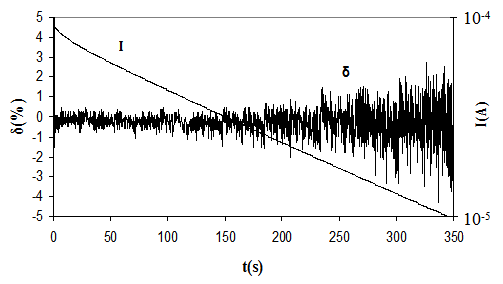 | Figure 2. Processes in D\A reactivity simulator, which operates in direct control mode direct control of DAC by continuous power signal with one current-forming resistor connected and one decade of the power signal variation |
In order to reduce this error the authors recommend the DAC-simulator [8] configuration given in figure 3. We use this diagram to illustrate the formation of a negative reactivity signal. In this configuration, the chosen interval of the power signal variation, which corresponds to the chosen reactivity, is preliminarily segmented and each of the segments corresponds to identical relative variation of this signal. For convenience, decadic segmentation is done. Data array is entered in the memory storage. This data consists of N serial decades as a set of digital codes. Thus each of decades is prenormalized on the given number А=2k by multiplication of the current values to value A/xi, where k is a number of DAC bits, xi is the value of power parameter at the beginning of i-th decade. Then a sequential sample of digital codes from the memory storage in program control unit is applied to the data-entry port Pdac. In order to reduce this error the authors recommend the DAC-simulator [8] configuration given in figure 3. We use this diagram to illustrate the formation of a negative reactivity signal. In this configuration, the chosen interval of the power signal variation, which corresponds to the chosen reactivity, is preliminarily segmented and each of the segments corresponds to identical relative variation of this signal. For convenience, decadic segmentation is done. 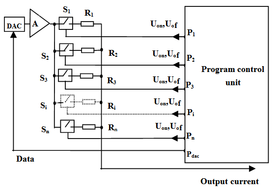 | Figure 3. D\A simulator with decadic switching of power parameter. A is the measuring amplifier; Si are electronic switches of current-forming resistors; Ri are the current-forming resistors; Pi are the ports for entry of keying signals; Pdac is the port of entry for control data of DAC |
Such types of control data arrays can be formed for any specified value of reactivity; therefore the changeover between two different simulator modes, i.e. changeover between different initial current and different reactivity values during signal formation, takes almost no time. This changeover reduces itself to a selection of a control data array from the memory and connection of one of the electronic switches of current-forming set of resistors (selection of initial output current).Figure 4 presents diagrams illustrating the simulator operation. It is shown that power parameter decades are normalized to the given value A (see vertical arrows in fig.4b) as the value of this parameter decreases (fig.4а) leading to a consequent change in the driving voltage level (fig.4c) and current forming resistance at t1, t2, t3,…, tN in the end of decades (fig.4d). As a result, the simulator output current forms (fig. 4e), which corresponds to the change in the power parameter of the reactor which controls the reactivity value. Diagram 4c shows that in this simulator the signal-to noise ratio at the output port of the measuring amplifier has the same value in all decades of its output signal variation because the measuring amplifier output signal varies within only one decade in all decades of output signal variation of the simulator.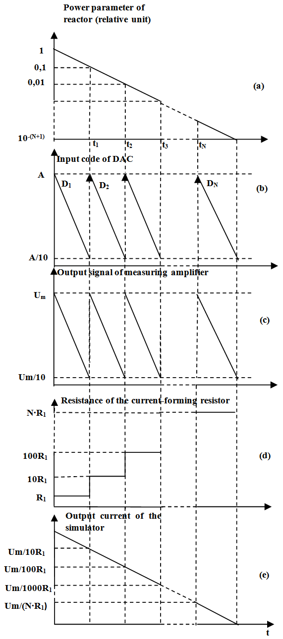 | Figure 4. Processes in D\A reactivity simulator designed according to the diagram on the fig.3 |
Another improvement of digital-to-analog applications for reactivity simulation problem is optimization of presentation of data stored in memory [9]. According to solution of the reactor kinetics equations, the reactor power for a fixed reactivity value begins to vary at an almost constant rate (one of the terms in the sum in the right-hand side of (2) becomes much greater than the others) at some moment after the reactivity jump.Therefore, a signal variation within intervals (decades) can be duplicated beginning from a certain interval (decades) when segmenting the simulator output signal variation into intervals (decades). The interval suitable for beginning of duplication and possible number of duplicated intervals (decades) is determined by admissible error of reactivity value which the reactivity meter calculates from the modified signal. The error can be estimated from solution of the reversed kinetics equation where reactor power is simulated by the modified signal. The performed calculations show that for practical reactivity values the error does not exceed 1% of the reactivity value, if the relative deviation of the simulated signal from the true one does not exceed 1% in each interval (decade) after the duplication.Therefore, programming of the memory device in DAC-simulator does not require recording all the information for the selected time interval of the power signal variation. Only part of this information is quite sufficient and, thus, less memory volume is required. To illustrate, we now compare similar diagrams given in figure 4 and figure 5. Let us consider in detail the diagrams for standard-memory DAC-simulator and DAC-simulator with "reduced" memory volume. For both cases, in practice the normalizing number A was 4095 corresponding to the maximal capacity of the 12-bit DAC based simulator.Obviously, for the standard-memory version, information about all decades of the power parameter variation should be stored in the simulator memory (see D1, D2…DN in fig. 4b). A different behavior is observed for "reduced"-memory DAC-simulator. Diagrams in figure 5 show simulation of the power signal corresponding to reactivity value of -0.1β. The input code generation (fig. 5b) uses the first decade of the power parameter variation, normalized to A (fig. 5a) for interval between 0 and t1 and the second decade of the power parameter variation, normalized to A for t1−t2, t2−t3, …, tN−T intervals, taking into account the second decade identity to all subsequent decades using constant ten-fold multiplier.In this case it is sufficient to store information only about two decades of the power signal variation in the simulator memory as it is shown by D1, D2,…, D2 (fig. 5b). The corresponding level variation of driving voltage (fig.5c) and resistance of current-forming resistor at the end of decades (fig.5d) is performed K-1 times during sampling of data corresponding to the end of the 1st decade (t1 moment) and N-K+1 times during sampling of data corresponding to the end of the second decade ( t2, t3…tN. moments), where N is the quantity of decades, K is the number of the decade where replacement of the actual signal by the duplicated one does not lead to a reactivity modeling error above 1%.For K=2 six-decade power signal variation case, the mentioned level changes are performed one time (K-1=2-1=1) and during selection of data corresponding to the end of the first decade and five times (N-K+1=6-4+1=5) during the selection of data corresponding to the end of the second decade. As a result, the simulator output current is formed (fig. 5e), which adequately represents the initial power parameter change for reactivity control using as little data as possible needed for the reactor power signal simulation.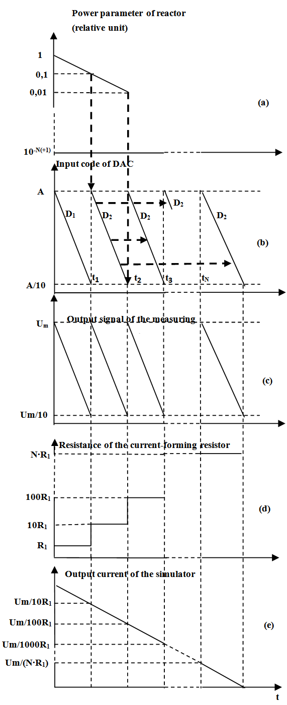 | Figure 5. Processes in D\A reactivity simulator with «reduced» memory storage |
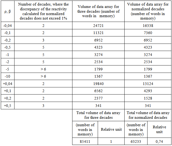
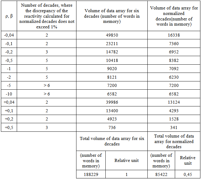
Since the reactivity simulator should provide a set of reactivity values characterizing for a task to perform (calibration or functional check of the reactivity meter), then each reactivity value corresponds to a specific K value, as it was mentioned before. Therefore, the reduction of the storage memory volume of the simulator as a whole is slightly lower than a similar reduction of data array calculated for one value of reactivity with a small absolute magnitude (±0.1β). As an example, for a practical set of reactivity values the above mentioned optimization of data provides 26 % and more than two-fold reduction of the memory volume for continuous simulation of reactivity in three and six decades of the power signal variation, respectively (see Table 1 and 2).Table 1. Comparison of standard and reduced memory volumes for three decades of power variation
 |
| |
|
Table 2. Comparison of standard and reduced memory volumes for six decades of power variation
 |
| |
|
3. Experiments
Figure 6 shows the time variation of the power signal and corresponding error of reactivity ρ=-0.1β modeled by the simulator shown in fig. 3. The simulation was performed in three decades of the power signal variation using the “reduced” memory 12-bit DAC based simulator. Let us note that the purpose of the current study was to obtain the value of error for reduce-memory DAC simulator as good as the value of error for analog simulator (≈1%). This problem has successfully been solved. It may be assumed that standard-memory DAC simulator would have much less error, but this fact wasn’t proved experimentally.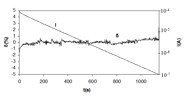 | Figure 6. Time history of current I and relative error δ of reactivity simulation ρ=-0.1β for D\A reactivity simulator with «reduced» memory storage |
Figure 7 shows similar diagrams for the case with direct control of DAC by continuous power signal with one current-forming resistor connected. The comparison between fig.7 and fig.6 illustrates advantages of the proposed methods as applied to D\A reactivity simulators.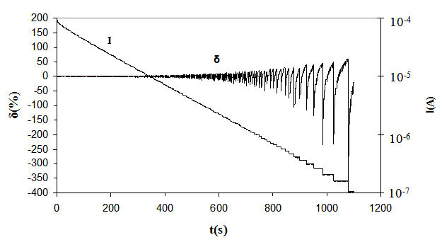 | Figure 7. Time history of current and relative error for simulation of ρ=-0.1β reactivity of direct control of DAC by continuous power signal with one current-forming resistor connected |
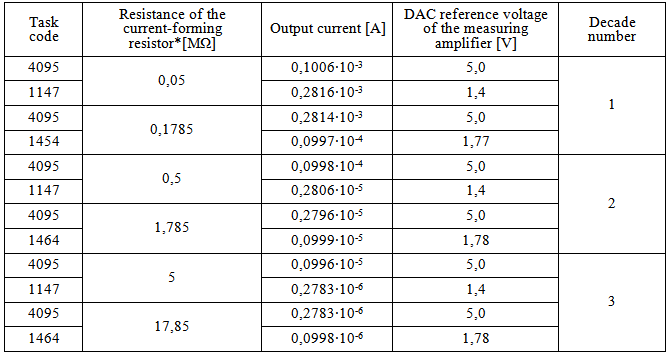
In particular, the diagram in figure 6 shows that the error of reactivity simulation exceeds 300% at the end of the third decade of the power signal variation. We also can see that this error exceeds ±1% even at the first half-decade as mentioned above. Based on this, it can be concluded that staying in the error range of ±1% using 12-bit DAC requires formation of the power signal by “sewing” of power signal variation half-decades with appropriate switching between current-forming resistors. Data given in fig.6 is obtained from «sewing» of six half-decades.Table 3 shows the current values of control codes for 12-bit DAC at selected points of half-decade «sewing» and corresponding values of current-forming resistor resistances and output currents.Table 3. Decadic sewing of 12-bit DAC
 |
| |
|
4. Conclusions
Testing of the described methods for designing D\A simulators of reactor kinetics and also methods for grouping and presentation of control data showed their advantages over traditional analog simulators. The D\A simulators are ready to use immediately after a change between operation modes and have almost invariable level of the relative deviation from its specified value in reactivity corresponding to DAC-simulator output signal. The deviation is within at least three decades of the power signal variation. Use of the obtained data in designing D\A simulators can significantly improve their performance characteristics.The authors would like to thank N.A. Vinogorov for his help with calculations and for precious comments.
References
| [1] | Yu. A. Kazansky, E.S. Matusevich. Experimental methods of reactor physics. М.: Energoatomizdat, 1984. p. 39. |
| [2] | R.R. Bagdasarov, V.A. Lititsky //Atomic Energy 1994. Vol. 76. Rel. 3. p. 171. |
| [3] | G.R. Kipeen. Physics of Nuclear Kinetics. М.: Atomizdat, 1967. p. 202. |
| [4] | V.F. Borisov, S.A. Gutov, V.V. Malokhatka. Patent № 2211485 RF, G06G 7/48, G 21C 17/06, G05B 15/02//Bulletin № 24. 2003. |
| [5] | A.L. Stolibko, Digital stabilizer of magnetic field, PTE №6, p. 26. 2013. |
| [6] | U.G. Manakov, Number-to-current converter of energy analyzer control system of magnetic spectrometer, PTE №4, p. 166. 2012. |
| [7] | U.V. Kolokolov, A.V. Monovskaya, Detection of bifurcation phenomena in dynamic PWM-converter, Elektrotehnika № 1, p. 43, 2013. |
| [8] | S.P. Dashuk, V.F. Borisov. Patent № 2244955 RF, G06G 7/54, G2 C 17/104//Bulletin № 2. 2005. |
| [9] | S.P. Dashuk, V.F. Borisov. Patent № 2287853 RF, G06G 7/54, G21C 17/104, G05B 15/02//Bulletin № 32. 2006. |
 Abstract
 Reference
 Full-Text PDF
 Full-text HTML