1. Introduction

The automotive industry has made significant technological progress over the last decade in the development of on-board control systems for improved car safety, handling, comfort, and preventing of dangerous situations[1-5]. All of the above-mentioned control systems can significantly reduce the number of road accidents, and these safety systems may be improved if the tire forces of the car are well known. However for both technical and economical reasons several fundamental variables (such as sideslip angle and tire forces) are not measurable in a large part of recent vehicles[6]. Consequently, these variables must be estimated or observed. The aim of this paper is to answer the question on how can the sevariables be deduced from knowledge of the vehicle’s states.

Since state estimators are usually based on the process model, they are sensitive to model inaccuracy. Consequently, vehicle modeling has been studied extensively[7-10]. Stephant, Charara, and Meizel[11] presented linear and non-linear estimation methods of vehicle sideslip angle based on the simple bicycle model and common lateral and yaw measurements. This model considered the deflection of tires and the suspensions of the vehicles. Kim[6], presented a methodology for describing lateral tire force dynamics based on the extended Kaalman filter (EKF) by studying vehicle dynamics. However, in order to simplify the EKF design, the estimation model was simplified to a four degree-of-freedom vehicle. A more complex model is the double-track (full-vehicle) model, which is a four-wheel model for studying the heave, pitch, yaw and roll motions[12-14].

In this paper, the vehicle state histories (i.e., longitudinal and lateral velocities, vertical displacements, vertical velocities, pitch angle, pitch rate, roll angle, and roll rate) and tire forces (i.e., longitudinal and lateral normal forces) are estimated by a methodology using an EKF[15-17]. The model used for the estimation synthesis is based on a ten degree-of-freedom vehicle model. The estimation results are validated by comparing these results with the data measurements collected from Carsim. Carsim is a model of the entire vehicle dynamics, comprised of suspension dynamics, lateral, vertical, and longitudinal motions, tire forces, and so on. Hence, the obtained simulation results can be considered to be very close to results of a real-car experiment. In addition, the observer uses as input the signals and measures available in the standard on vehicles equipped with driving assistance systems such as ABS and ESP. With accurate estimation of the tire forces and the instantaneous tire-road friction coefficients for the current road condition, the performance of the car can be improved by optimization of either acceleration or braking for various road conditions. This estimate results can be used to give the driver or a closed-loop controller an advance warning of the approaching tire force limit.

The outline of this paper is as follows: in Section 2 a ten degree-of-freedom (DOF) nonlinear full-vehicle model is derived. The vehicle state histories and tire forces are explored in Section 3. The estimation results are validated in Section 4 by comparing these results with the data measurements collected from Carsim. Conclusions are given in Section 5.

2. Nonlinear Full-Vehicle Model

Figures 1 and 2 show the full-vehicle model: horizontal model, vertical model, and tire model[18]. The heave, pitch and roll motions of the vehicle body are included. The lateral and longitudinal velocities of the vehicle ( and , respectively) and the yaw rate, , constitute the three DOF related to the vehicle body at the center of gravity (c.g.) as depicted in Figure 1. This model obtains the longitudinal and lateral tire forces from the tire model. Based on these two forces, the horizontal model calculates the horizontal performance of the vehicle. The vertical model of a vehicle is made of seven DOF and four DOF of the four wheels, as depicted in Figure 2.

In the horizontal vehicle model shown in Figure 1, V is the vehicle velocity, is the yaw rate, is the side slip angle, and is the front wheel steering angle. The lengths and refer to the longitudinal distance from the c.g. to the front wheels and to the rear wheels, respectively, and is the lateral distance between left and right wheels (track width). Let the longitudinal and lateral tire forces be given by and , respectively, and is the slip angle of the wheel. The superscript or subscript indicates the front and rear, while the superscript or subscript indicates the left and right tires, respectively. Then the equations of motion of the vehicle body are

(1)

(2)

(3)

where is the vehicle mass, is the moment of inertia of the vehicle about its yaw.

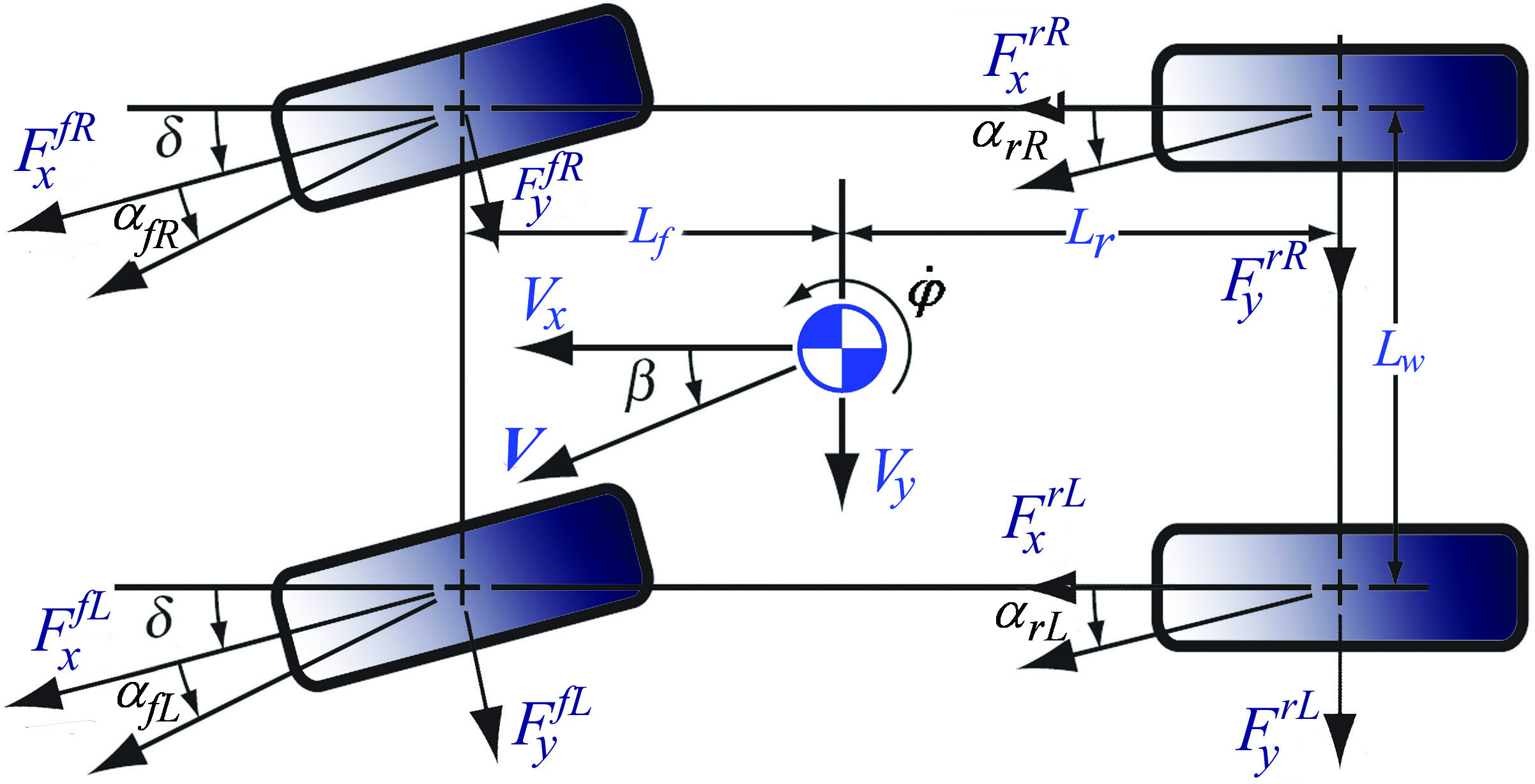Figure 1. Three degree-of-freedom full-vehicle model

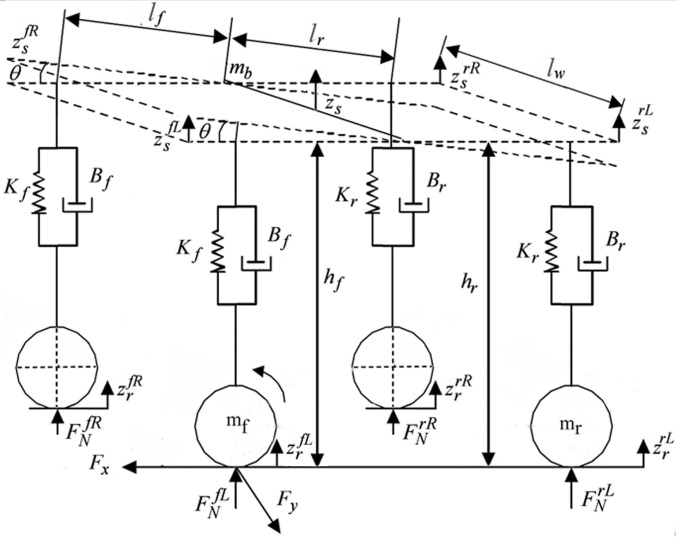Figure 2. Eleven degree-of-freedom full-vehicle model

In the vertical model and the tire vehicle model shown in Figure 2, let and are the vertical displacement of the body at the center and the corner, respectively, the road profiles, is the body pitch angle, is the mass of the vehicle without the mass of the front and rear wheels , is the normal tire force, and is the vertical distance from the c.g. to the center of the front and the rear wheel at equilibrium. The spring and damping constants and , respectively, are the lumped parameters associated with the passive suspension system. For a small value of , after applying a force-balance analysis to the model in Figure 2, the equations of motion can be derived to the static equilibrium positions. The equations for describing the sprung mass are

(4)

(5)

(6)

where with being the roll angle. In the models (5) and (6), and are the moments of inertia of the vehicle about its pitch and roll axis, respectively. From (1) to (6), we defined the state vector as

, (7)

and the measurement vector as , which incorporates all the measurement values, and input vector . and are the longitudinal and lateral accelerations of the vehicle.

3. Estimation of Tire Forces

The EKF is dedicated to the estimation of the state vector of nonlinear systems[15]. In order to develop directly a discrete-time EKF, the dynamic continuous evolution of the vehicle (1) to (6) has to be discretize. This discretization is performed by a forward Euler approximation. A nonlinear discrete-time system is obtained in the form:

(8)

where is the estimated state vector, is the reconstructed output, which is composed of the tire forces and vehicle state histories, is the input vector, are the eight estimated tire forces, is the dynamic noise vector, and is the measurement noise vector. Both of the noise vector are supposed to be non-intercorrelated, stationary, white and Gaussian with known covariances. The covariances of and are noted as and , respectively. Here the tire forces are considered as parameters that have to be estimated at the same time as the state. They will therefore be included directly in the state vector. As parameters, the tire forces have no dynamics and are modeled with a derivative equivalent to a random noise. To model each of the tire forces, the following model form[19] is used.

(9)

where is the force, and are first and second derivatives of the force, respectively.

In (8) the nonlinear function relates the state vector and the input vector at time step to the state at time step . The measurement vector relates the state to the measurements . Vectors and denote the superimposed process and measurement noise, respectively. The variance of and are Q and , respectively. The control inputs and the outputs are measured using a set of sensors. All of these sensors are assumed to be on the vehicle. The state vector and the output vector are Gaussian even though they are conditioned on the measurements from time step 1 to time step . is the mean of the state vector conditioned on the measurements from time step 1 to time step with as its covariance. The variables and are also, respectively the estimate and estimation error covariance provided, at each time step, by the EKF.

The EKF algorithm is recursive and operates in two steps. They are the prediction step and the update step. The prediction step consists of the propagation of both the state estimate and the state estimation error covariance between two sampling instants, as follows.

(10)

(11)

where is the forecast, is the prediction error covariance and is the dynamic matrix resulting from the linearization of the state equation around the estimate . The update step occurs at each sampling time, and consists of the corrections against the measurement state forecast, and the prediction error covariance, as follows.

(12)

(13)

(14)

where results from the linearization of the output equation around the forecast. The vehicle speed, longitudinal and lateral accelerations, and yaw rate are measured by an inertial sensor and the steering angle is measured by a steering sensor. The filter is initialized with a state estimate corresponding to the true state and a large covariance matrix.

To ensure the observation of the parameters using the two measurement sets presented above, an observability study was performed to show that our system was observable. This observability study is made by calculating the rank of the observability matrix which is given by the derivative of the nonlinear system:

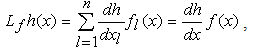(15)

where iteratively and . The observability matrix for a nonlinear system is then given by

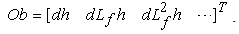(16)

If the observability matrix is invertible at the current state and input, the system is observable. This matrix is invertible as its Jacobian matrix has a full rank. The tire model is used to simulate the true tire forces of the vehicle. Using the estimate vectors, the front and rear normal forces at the tire-road interface are as follows:

(17)

whereis the gravity acceleration.

4. Simulation and Discussions

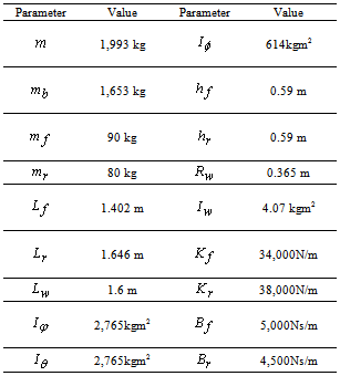
In this paper, the simulation model is a ten degree-of-freedom of a full-vehicle model that includes vertical suspension dynamics, roll, yaw and pitch motion. Using the vehicle speed, yaw rate, longitudinal and lateral accelerations of the vehicle at c.g. As the measurement vectors, the steering angle, and the braking as input control, the vehicle state histories and tire forces variables were estimated. The vehicle parameters for the Carsim and simulation are given in Table 1. Using equation (16), the observability matrixwas invertible at the current state and input as its Jacobian matrix has a full rank, hence the system was observable. Then, the estimated results were compared with the obtained responses from the Carsim. Figures 3 - 7 show the comparison of the results obtained from the Carsim and the estimated values using an EKF algorithm.

Braking and control systems must be able to stabilize the vehicle during cornering. When the vehicle is subjected to transversal forces, the tire torsional flexibility produces an aligning torque which modifies the vehicle body motion and the original tire direction. Hence, the signals of the pitch, roll, yaw, and sideslip angle are important in determining the stability of the vehicle. Measuring these variables, especially the sideslip angle, using the sensor would represent a disproportionate cost for the car industry, so they musttherefore be observed or estimated. Thus, Figure 3 shows the estimated pitch, roll, yaw, and sideslip angle.

Table 1. Vehicle Parameters

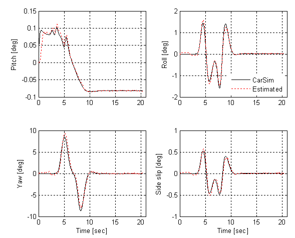Figure 3. Carsimand estimation for and

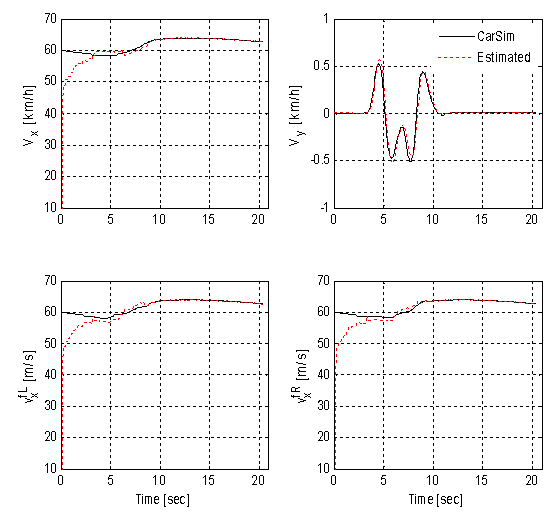Figure 4. Carsim and estimation for and

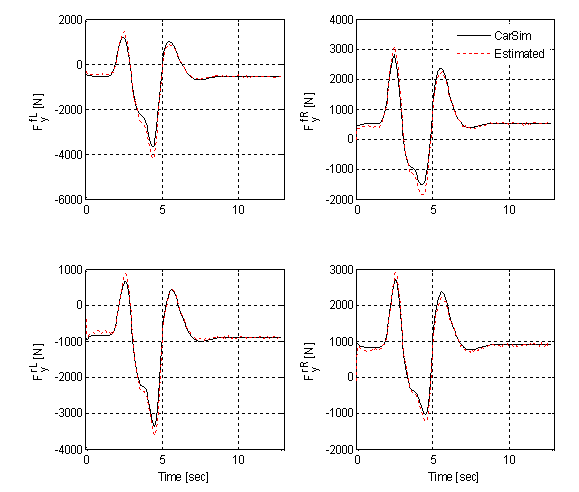
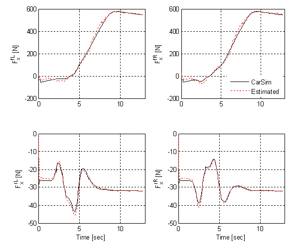Figure 5. Carsim and estimation for

Figure 6. Carsim and estimation for

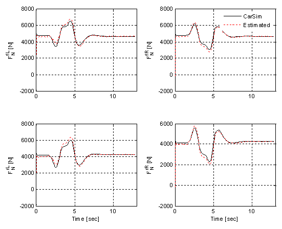Figure 7. Carsim and estimation for

As the figure shows, the estimated values and the responses obtained from the Carsim are in good agreement. Figure 4 shows that the longitudinal andlateral vehicle velocities at c.g. as well as the longitudinal wheel velocities (front left and front right) are similar to those obtained from the Carsim. This estimation study proves that the mathematical model developed above can give a good evaluation of the real dynamics of a vehicle. disturbances from a road are transmitted through the tires, the information of the tire behavior is very important. The longitudinal, lateral, and normal tire forces are given in Figures 5 – 7, respectively. It can be seen that the estimates are quite close to the exact force computed by the Carsim. The small negative bias present in the longitudinal tire forces is caused by the other forces not taken into account in this work (such as the drag force and the rolling resistance). Since the tire forces are not modeled at all, uncertainty is very high and is represented by a high noise level. On the other hand, since the simulation is noise free, the noise on the observations is said to be quite small. Of course, in a real car, those characteristics could change depending on the specifications on the sensors.

5. Conclusions

In this paper, aten degree-of-freedom full-vehicle nonlinear model was derived. The EKF was used in order to estimate the vehicle state histories and the tire forces. Simulations showed that the estimation errors achieved by the EKF are acceptable. EKF showed fast convergence using only four measurements (i.e., vehicle speed, longitudinal and lateral accelerations, and the yaw rate) of the dynamic state vector. The comparison between the estimated results and the obtained from the Carsim confirmed the validity and accuracy of the model, in which all the state variables followed the Carsim responses well. The sideslip angle, which is an important parameter to measure vehicle stability, is usually measured by a specific sensor, which it is too expensive to be equipped on an ordinary vehicle. Thus, this variable was estimated in this paper by using the estimated dynamic state, and the estimation error was found to be very small. Therefore, the expansive sensor can be replaced by a virtual estimator to calculate the sideslip angle.