1. Introduction

Aircraft Flight control systems consist of flight control surfaces, cockpit controls, connecting linkages and necessary operating mechanisms to control an aircraft’s direction in flight. Aircraft engine controls are also considered as flight controls as they change speed. They can be divided in to three main groups:

-Primary Flight Control

-Secondary Flight Control

-Auxiliary Flight Control.

An aircraft flight control system is highly complex, dynamic, and nonlinear and contains a significant amount of hysteresis. Parallel cascade identification is well suited to cope with reduced number of real data signals. A new faster method of producing flight control models is proposed in a black box manner, using only input and output data from the flight control system and ignoring the system's physical structure almost entirely.

The aileron flight control system poses significant challenges to black box identification methods since it has nonlinearities of high order is dynamic and contains significant hysteresis. The parallel cascade method of system identification used is however able to handle these challenges. A simulation using a traditional flight control mode1 is used as the system whose behavior is to be reproduced by the parallel cascade model. The criteria used by the U.S. Federal Aviation Authority are to certify commercial Full Flight Simulators.

The paper focuses on the main unknown remains to what extent the simulator environment reflects in the-air conditions and to what extent this is required to achieve a certain training or test objective. First, the simulator is only as good as the data it contains i.e. the quality of the model representing the aircraft and the flight environment to be simulated. Secondly, inherent limitations of the system used to simulate can be the cause of mismatches. The motion system of a simulator does posses one of the most obvious constraints with its very limited amount of travel. Fortunately, the pilot can be made to perceive the motion desired if the main cues are correctly simulated, allowing for some deviation in the others.

2. Aircraft and Flight Simulation Overview

An aircraft simulation that allows pilots to start training to fly the new aircraft without ever having set foot in it. This kind of device is known as a Full Flight Simulator (FFS). FFS is meant to simulate the environment of the aircraft cockpit and behavior of the aircraft with accuracy requires that the visual, aura and tactile inputs which the pilot receives, whether from the aircraft systems or the environment or both be simulated realistically. Additionally it must run in real-time.

A main concern is the speed at which the model can be run; since the simulator must run in real-time and at a high enough iteration rate that the effects seem real. In most cases a tradeoff between accuracy and complexity must be negotiated. The primary simulator components make up the pilot-in-the-loop of the FFS where the pilot provides the inputs to the simulator and receives a feedback response through his or her hands, eyes, ears and "seat-of-the-pants". These systems are: the flight controls. e.g. the pilot control stick wheel and rudder pedals and flight control models, through which the pilot provides inputs to the simulator: the aerodynamic model which computes the effects of those inputs on the aircraft; the visual system which provides the visual feedback on the airplane behaviour and the environmental conditions: the motion system which gives feedback on the behaviour of the airplane with motion and acceleration cues; and the flight control (again) which provides feedback to the pilot's hand. There are also many secondary and auxiliary systems that require simulation including secondary flight control systems such as the flap system and the throttle controls.

2.1. Aircraft Flight Control Simulation using Parallel Cascade System

Microsoft's Flight Simulator gives an onscreen representation of an aircraft instrument panel and a view of the scene in front of the aircraft, while a joystick provides the "pilot" with control over the simulated aircraft. Full Flight Simulator replicates the appearance of the aircraft cockpit, the functionality of almost al1 the aircraft's systems. its aerodynamic behavior, the tactile (feel) cues from the light controls, the acceleration (motion) cues and the visual cues from the scene in front of the aircraft. These FFS are multi-million dollar, custom made devices that rely on an array of powerful computers and electrical, mechanical, pneumatic and hydraulic systems to produce the simulated environment.

Basic requirements to be considered as a suitable software model are as follows:

i. The behavior of the real flight control system can be reproduced by the simulation system to meet the predatory requirements;

ii. It can be run at a high enough iteration rate to be used in a Full Flight Simulator;

iii. The required outputs for implementation with the standard hydraulic servo-electric actuator controllers are produced: and

iv. It must accept the appropriate inputs from other systems and provide the appropriate outputs.

2.2. Identification of Aircraft System Models

Two of the most common methods include

(1) Identification of transfer functions from test input and output data

(2) Physically based models.

2.2.1. Identification of Transfer Functions

The identification of transfer functions is “The inverse problems of the second type". It requires the collection of test data from the aircraft and then the determination of the frequency response of the system. This method can be described as a "black box" method in that only input and output data are used to find the model. The flight test can be performed either by oscillating the elevator about its trim position at various frequencies or by applying step or pulse motions to the elevator. In both cases the elevator angle. The response of the steady-state angle of attack (the angle of the aircraft from horizontal relative to its direction of motion) and the pitch-rate are measured.

The first method produces the frequency response of the longitudinal motion of the aircraft directly. The second method requires that the transfer function be computed in some way. For instance, from Fourier transform of the output and input signals. Once these frequency response curves have been obtained, an equation of the following form

G (jω) = (a +b jω) / (A +Bjω –ω2)

Where:

G (jω) is the transfer function of pitch control input to pitch-rate.

J is the imaginary number *- 1.

ω is the angular frequency.

a, b, A, B are real parameters formed from inertia constants and stability derivatives.

This method works if the system is nearly linear and if a second order differential equation is well suited to the system being identified. The transfer function describes the input of the control stick to the longitudinal motion of the aircraft. However, the control stick input is only the primary input into this aspect of the aircraft behaviour.

2.2.2. Physical Models

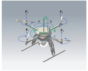Figure 1. Quad rotor Model

The results of simulations are in two sections: first – inner loop control with all types of PID controllers; second – performed in the cascade control system. The aerial vehicle consists of a rigid cross frame equipped with four rotors as shown in Figure 2. The two pairs of propellers turn in opposite directions. By varying the rotor speed, the lift force can be changed and motion created. Thus, increasing or decreasing the four propellers’ speeds together generates vertical motion. Changing the opposite propellers’ speed conversely produces roll rotation coupled with lateral motion. Pitch rotation and the longitudinal motion result from 1 and 3 propellers’ speed being conversely modified. Yaw rotation is a result of the difference in the counter‐torque between each pair of propellers.

3. Flight Simulation Issues

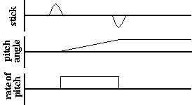
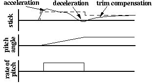
The most common error encountered in flight simulation involves the issue of the level of modeling chosen for the simulation. Consider the issue of stability. When you pull back on the stick from level flight, and hold the stick slightly of center, the nose begins to rise, and the plane begins immediately to climb. As the nose rises the airspeed begins to decay very slowly and almost imperceptibly, and as this occurs, the rate of climb also falls off. Due to the inherent longitudinal stability, this reduced airspeed has the effect of changing the trim to more nose-down, so that with the stick held steady, the rate at which the nose rises begins to decay. If held long enough, the pitch attitude will eventually equilibrate at some nose-up angle, at a reduced airspeed, and at a rate of climb much smaller than that experienced when the climb was initiated, as suggested in Fig 2.

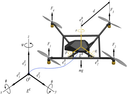Figure 2. Aircraft Orientation using Euler Angles

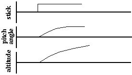Graph 1. Stability Control

The pilot's psychological conception of the action of the elevator control is rather different however, since he generally thinks of the stick as controlling the pitch altitude, as suggested in Figure 3, i.e. he pulls back until the nose reaches the desired climb altitude and then returns the stick to the neutral position for the steady climb.

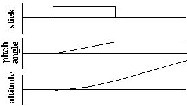Graph 2. Elevator Control

There are even more complex and subtle effects such as the rotational inertia as the aircraft begins to rotate in pitch, so that to initiate a pitching-up at a constant rate, one would actually have to give an initial pulse of stick-aft, followed by neutral stick as the nose rotates upwards until the desired pitch angle is attained, at which point a pulse of stick-forward would be required in order to stop the upward rotation and maintain the pitch at the new climb angle, as suggested in Figure 4.

Graph 3. Pitch Control

This rotational inertia effect is superimposed on the other effects, and again is totally unconscious, so that in order to perform the constant-rate pitch-up depicted in Figure 3, the actual control input would be something like Figure 5.

Graph 4. Actual Control Input

Figure 3. Second Order Differential System Block diagram

Figure 4. Cascade Control

Figure 5. Aircraft Cascade Loop Control

4. Formulation of Differential Equations

The formulation of differential equations for mechanical systems begins with the concepts of mass, inertia and particle dynamics (Newton’s Laws of Motion). Rotational dynamics and conservation of momentum are also used as appropriate. Ryswick and Taft describe a four step procedure for the formulation of the differential equations that describe the dynamic system:

1. System definition:-procedure using free body diagrams.

2. Isolation of each rigid body: - external forces and reactions

3. Formulation of differential equations: - apply the equilibrium equations of d'Alembert to each rigid body:

∑F_ext + F_i = O (in any direction)

Where:

Fe, are the external forces applied to the system and

F is inertial force.

4. Equation reduction: - using matrix manipulation techniques.

These free bodies can be joined together to form layer complex systems and additionally nonlinear and or time-varying structures can be included. Nonlinear effects are very difficult to mode1 in this way as the determination of the system equations becomes cumbersome. However this method can deal with nonlinearities in an ad hoc manner.

Damping force = Velocity*Damping constant

Spring force = Position*Spring constant

Acceleration = (Input force – Damping force –

Spring force)* 1 /Mm:

Velocity += Acceleration*Time constant'

A first order exact differentiator is used in order to estimate the virtual control inputs, which simplifies the control law design. In addition, the wind parameter resulting from the aerodynamic forces is also estimated in order to ensure robustness against these unmatched perturbations. The performance and effectiveness of the proposed controller are tested in a simulation study taking into account external disturbances. The design of a controller based on the block control technique combined with the super twisting control algorithm for trajectory tracking of a quad rotor helicopter.

5. Cascade and Parallel Cascade Models

Many nonlinear systems can be modelled as a sum of cascades each of which approximates a portion of the system. Each cascade comprises alternating dynamic (i.e. finite memory) linear (L) and static (i.e. memory less) nonlinear (N) elements. They can be abbreviated LNL, NLN, and LN. etc. depending on the type and order of the elements.

Other forms of cascades are possible. Simpler versions include LN and NL cascades, which are known as Wiener and Hammerstein models respectively. While Hammerstein models can be used to approximate only a narrow class of nonlinear systems. Wiener models can be used to approximate a very wide class of nonlinear systems. Kornberg IKOR82, KOR90. KOU91 1 showed that any system having a Wiener functional expansion could be approximated to an arbitrary degree of accuracy by a sum of LN (Wiener model) or LNL cascades developed one at a time. He also showed that a finite sum of LN cascades could exactly represent any discrete-time finite-memory, finite-order.

MSE, the error in a designed experiment, σ ², is the natural variation in the response when one of the experimental combinations is replicated. One important challenge in a designed experiment is obtaining an unbiased estimate of σ ². Too often, experimenters do not realize the impact that data collection and analysis assumptions have on the estimate of σ ². If the estimate is biased, tests of the effects in the analysis will be adversely affected. It is important to carefully inspect the data collection and model reduction process for signs of bias in MSE before the results are used to reach any conclusions. To avoid a biased MSE term, statistically valid model- reduction techniques should be used and the experiment should be properly randomized.

The individual cascades are identified in two stages. First the impulse response of the dynamic linear element is defined using a slice of a first- or higher-order cross correlation of the input with the residue. The output from the dynamic linear element is then the input to the static nonlinear stage for which a polynomial is best-fit to minimise the MSE of the residue. These impulse responses and polynomials form the individual LN cascade models and are used to determine the residue for the next cascade to be identified. This process is continued until the MSE of the residue is sufficiently small or no further meaningful reduction is obtained by further cascades. Cascade paths that are identified can be evaluated as to their effectiveness in terms of MSE reduction and used or discarded appropriately.

5.1. Obtaining the Cascade Output

Once the polynomial coefficients have been found, the cascade output is found. The individual cascade outputs are then summed to get the final output. In order to avoid numerical overflow and underflow problems that can result with such high order polynomial elements it is important to normalise the input and output data. In order to use the parallel cascade method with a reasonably small memory length in the dynamic linear element while running the model at a high sampling (iteration) rate. The data is simply sampled at the high rate but only every n-th sample is used to calculate the linear element's output at any particular instant, where n is the ratio of the higher sampling rate to the parallel cascade model rate.

5.2. Extracting the Output Derivatives from the Parallel Cascade Mode1

Graph 5. Time Vs Control Simulation

The identified parallel cascade model can be modified and used to compute the derivatives of the output directly from the input. This can be done using the chain rule and finding the differentials of the static nonlinear polynomial element in cascade. Therefore Kornberg’s method of parallel cascade system identification outlines parallel cascades, in which the individual cascades are identified one at a time and each consists of two elements. The first element is a convolution of the input with an impulse response where the impulse response is found by cross correlation of the input and the current residue. The second element is a polynomial (whose input is the output of the first element) which is best fit to the residue in a minimum MSE sense.

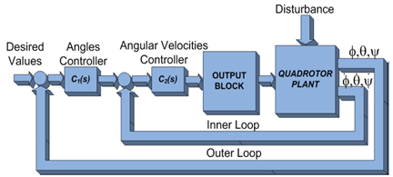
6. Cascade Control Scheme

In control applications, the rejection of external disturbances and performance improvement are major concern. In order to fulfill such requirements, the implementation of a cascade control system can be considered .Basically, in a cascade control scheme the plant has one input and two or more outputs. This requires an additional sensor to be employed so that the fast dynamics can be measured. The primary controller and the primary dynamics are components of the outer loop. The inner loop is also a part of the outer loop, since the primary controller calculates the set point for the secondary controller loop. Furthermore, the inner loop represents the fast dynamics, whereas the outer should be significantly slower (with respect to the inner loop). This assumption allows interaction that can occur between the loops to be restrained, improving stability. Therefore, a higher gain in the inner loop can be adopted. An additional advantage is that the plant nonlinearities are handled by the controller in the inner loop, and exert no meaningful influence on the outer loop .

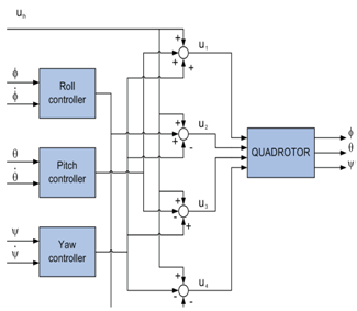Figure 6. Quadrotor Control

The main goal of the output block is to accomplish an algorithm of quadrotor control, and provides decoupling of control channels in steady state. The control inputs from cascade controllers, about each axis are therefore combined to generate the control inputs u1 through u4, for motors 1 to 4.

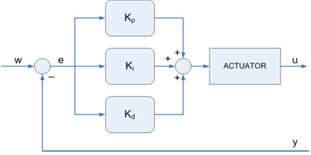
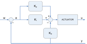
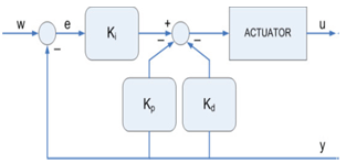
6.1. PID Controller Types

PID Controller-type A

In control theory the ideal PID controller in a parallel structure is represented in the continuous time domain as follows:

u(t) = K_p e(t) + K_{i 0}ʃ^t e(τ) dτ+K_d de(t)/dt

Where:

Kp ‐ proportional gain,

Ki ‐ integral gain,

Kd ‐ derivative gain.

Figure 7. Type A PID Controller

The problem with conventional PID controllers is their reaction to a step change of the input signal, which produces an impulse function in the controller action. There are two sources of the violent controller reaction – the proportional term and the derivative term. Therefore, there are two PID controller structures that can avoid this issue.

PID Controller – type B

It is more suitable in practical implementation to use the derivative of output controller form . The equation of the type B controller is:

u(t) = K_p e(t) + K_{i 0}ʃ^t e(τ) dτ - K_d dy(t)/dt

If PI‐D structure is used, discontinuity in r(t) will still be transferred through proportional into control signal, but it will not have as strong an effect as if it was amplified by derivative element.

Figure 8. Type B PID Controller

PID Controller – type C

Figure 9. Type C PID Controller

With this structure the transfer of reference value discontinuities to control signal is completely avoided. Control signal shows less sudden changes than with other structures.

Test Requirements

Roll (Aileron) Control Static Test:

2 1b breakout (notch) force +/- 3 lb or +/- 10% elsewhere

Dvnamics at 1l primary controls:

+/- 10% time to 1st zero crossing

+/- (n+l)* 10% of the period thereafter for the n-th overshoot

+/- 10% amplitude of 1st overshoot

+/- 20% amplitude of the 2nd and subsequent overshoots greater that 5% of initial displacernent

+/- 1 overshoot

6.2. Time History of Pitch angle and Angular Velocities

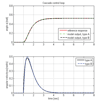Graph 6. Pitch Angle Vs Angular Velocity

These results show that the basic requirements targeted in this thesis for implementation of a new flight control system simulation in an FFS are met. Namely that:

1) The behaviour of the flight control system can be reproduced to within the FAA tolerances using parallel cascade models

Proof: Fault tolerance is designed into the system by the use of stringent processes and rules. A uniform distribution of increased local stresses in stiffeners and skin at the ends of the adapters was a major cause of almost simultaneous initiation of several cracks. These cracks were growing at nearly equal rates. In all cases the parallel cascade model was able to simulate the behavior of' the aircraft flight control system to within the tolerances set by the FAA for full flight simulators. These tests included three different sampling rates and additional tests were performed to test the robustness of the parallel cascade model in the presence of input noise. The magnitude of the initial overshoot is improved from 9.9% to 3.1% difference (the tolerance is 10% difference)

2) The parallel cascade model can be run at a high enough iteration rates to be used in a Full Right Simulator:

Proof: In order to use the parallel cascade method with a reasonably small memory length in the dynamic linear element while running the model at a high sampling (iteration) rate the data is simply sampled at the high rate, but only every n-th sample is used to calculate the linear element's output at any particular instant, where n is the ratio of the higher sampling rate to the parallel cascade model rate. The memory of the dynamic linear elements was chosen to match the length of the dynamic response of the flight control system, which was 1.45 seconds or 87 samples at the 60 Hz sampling rate used.

3) The required outputs for implementation with a PID hardware controller are produced:

Proof:Simulation hardware systems consist of hydraulic or electric load unit or jacks These require electrical controllers to provide the required performance from the load units and the controller most commonly used in industry are simple proportional, integral, differential (PID) controllers. For such a controller to function it must be supplied with three signals. i.e. the position, the velocity and the acceleration.

4) The system is stable with respect to additive input noise of appropriate levels:

Proof: An aircraft flight control simulation system must be stable under al1 conditions in order to ensure the safety of the simulator operator. The flight control simulation system hardware is capable of generating high forces and velocities. Therefore an unstable system could impart significant kinetic energy to the operator and cause physical injury. Various safety measures are used to avoid this consequence. However it is clearly necessary that the software model driving the hardware be stable. There are various intentional sources of noise that are used to simulate aircraft conditions. For example turbulence which is felt by the pilot through the control response and the model must be stable under these conditions. Noise was added to the input force signal. The noise used was pseudo Gaussian and filtered through a 50 Hz low pass filter to approximate the input frequency cutoff of a typical hydraulic actuator powered flight control system These noise studies were used to determine model stability only and no comparison to the actual model behavior under noisy conditions was done. The results were compared to the noiseless behavior of the flight control model to illustrate the general stability of the parallel cascade model under these conditions.

7. Significance

This paper showed that parallel cascade models could be used to reproduce the behaviour of an aircraft flight control system. One particular aspect of the control behaviour was looked at namely, the response of the control to the pilot input. Parallel cascade system identification has been used to model the physical behaviour of any pan of a flight control system and the first time that the method has been shown to work when identifying the behaviour of systems with significant hysteresis.

Simulation Graphs:

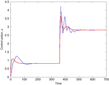Graph 7. Time Vs Control Action

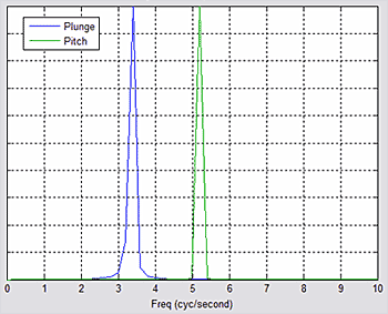Graph 8. Frequency Characteristics

8. Conclusions

In this paper the cascade control structure is proposed as a solution to control tasks formulated as angular stabilization. The angular velocities of the rotating platform are additional measurements that can be used in the inner loop. In this case, there is no need to assemble any extra sensors, and the AHRS (Altitude and Heading Reference Signal) therefore provides not only angles but also other raw data, such as accelerations, angular velocities and gravitational field strength. The outer loop is based on the Euler angles and the measurements are calculated from the combination of the accelerometers, gyroscopes and magnetometers. The conducted simulations and analysis proved the ability of the designed cascade structure in controlling the orientation platform angles and providing the promising fundamentals for practical experiments with a physical plant. The cascade PID control system can be introduced together with the requirements and appropriate constraints for the system to validate such control algorithm applications in real conditions.

9. Future Work

The complete Flight control system is not simulated and requirement is limited to accepting inputs only in terms of direct pilot inputs and other inputs that can be considered to be additive to the pilot input. e.g. aerodynamic turbulence modeled as input noise. The outputs of the model are limited to the primary output of the portion of the target flight control system modeled: the control position, velocity and acceleration. Higher order differential equations modeling are difficult.