-
Paper Information
- Paper Submission
-
Journal Information
- About This Journal
- Editorial Board
- Current Issue
- Archive
- Author Guidelines
- Contact Us
International Journal of Instrumentation Science
p-ISSN: 2324-9994 e-ISSN: 2324-9986
2013; 2(2): 13-24
doi:10.5923/j.instrument.20130202.01
Calculation of Full Energy Peak Efficiency of NaI (Tl) Detectors by New Analytical Approach for Cylindrical Sources
 Abstract
 Reference
 Full-Text PDF
 Full-text HTML
Ahmed M. El-Khatib, Mohamed S. Badawi, Mona M. Gouda, Sherif S. Nafee, Ekram A. El-Mallah
Physics Department, Faculty of Science, Alexandria University, Alexandria, 21511, Egypt
Correspondence to: Mona M. Gouda, Physics Department, Faculty of Science, Alexandria University, Alexandria, 21511, Egypt.
| Email: |  |
Copyright © 2012 Scientific & Academic Publishing. All Rights Reserved.
A new analytical approach for calculation of the full-energy peak efficiency of NaI (Tl) is deduced. In addition, self attenuation of the source matrix, the attenuation by the source container and the detector housing materials are considered in the mathematical treatment. Results are compared with those measured by two cylindrical NaI (Tl) detectors with Resolution (FWHM) at 662 keV equal to 7.5% and 8.5%. 152Eu aqueous radioactive sources covering the energy range from 121 keV to 1408 keV were used. By comparison, the calculated and the measured full-energy peak efficiency values were in a good agreement.
Keywords: Nai (Tl) Scintillation Detectors, Cylindrical Sources, Full-Energy Peak Efficiency, Self-Attenuation
Cite this paper: Ahmed M. El-Khatib, Mohamed S. Badawi, Mona M. Gouda, Sherif S. Nafee, Ekram A. El-Mallah, Calculation of Full Energy Peak Efficiency of NaI (Tl) Detectors by New Analytical Approach for Cylindrical Sources, International Journal of Instrumentation Science, Vol. 2 No. 2, 2013, pp. 13-24. doi: 10.5923/j.instrument.20130202.01.
Article Outline
1. Introduction
- NaI (Tl) detectors are commonly used to identify and measure activities of low-level radioactive sources. They have high detection efficiency and operate at room temperature[1]. The determination of the activity for each radionuclide requires prior knowledge of the full-energy peak efficiency at each photon energy for a given measuring geometry, which must be obtained by an efficiency calibration using known standard sources of exactly the same geometrical dimensions, density, and chemical composition of the sample under study. Standard radioactive samples, if available, are costly and would need to be renewed, especially when the radionuclides have short half-lives[2]. In addition, the influence of the source matrix on the counting efficiency can be expressed by the self-attenuation factor, describing the fraction of gamma-rays not registered in the full-energy peak due to scattering or absorption within the sample[3]. An effective tool to overcome these problems could be the use of computational techniques[4-9] to complete calibration of the gamma spectrometry system. Also, Selim and Abbas [10-14] solved this problem by derived direct analytical integrals of the detector efficiencies (total and full-energy peak) for any source-detector configuration and implemented these analytical expressions into a numerical integration computer program. Moreover, they introduced a new theoretical approach[15-17] based on that Direct Statistical method to determine the detector efficiency for an isotropic radiating point source at any arbitrary position from a cylindrical detector, as well as the extension of this approach to evaluate the volumetric sources.In the present work, authors will modify this simplified approach to determine the full-energy peak efficiency of the co-axial detector with respect to point and volumetric sources, taking into account the attenuation by the dead layer (reflector) and the end-cap material of the detector, the self attenuation by the source matrix and finally, the attenuation by the source container material.
2. Mathematical Viewpoint
2.1. The Case of a Non-axial Point Source
- Consider a right circular cylindrical (2R × L), detector and an arbitrarily positioned isotropic radiating point source located at a distance h from the detector top surface, and at a lateral distance ρ from its axis. The efficiency of the detector with respect to point source is given as follows[16]:
 | (1) |
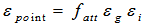
2.1.1. The Intrinsic ( εi ) and the Geometrical ( εg ) Efficiencies
- The intrinsic and geometrical efficiencies are represented by Eqs. (2) and (3) respectively.
 | (2) |
 | (3) |
 is the average path length travelled by a photon through the detector, Ω is the solid angle subtended by the source-detector and they are represented by Eqs. (4) and (5) respectively. μ is the attenuation coefficient of the detector material.
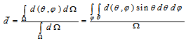 | (4) |
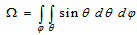 | (5) |
|
2.1.2. The Attenuation Factor ( fatt)
- The attenuation factor fatt is expressed as:
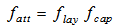 | (6) |
 and
and  are the attenuation factors of the detector dead layer and end cap material respectively and they are given by:
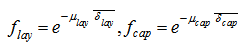 | (7) |
 and
and  are the attenuation coefficients of the detector dead layer and the end cap material, respectively. While
  and
and  are the average path length travelled by a photon through the detector dead layer and end cap material, respectively. They are represented as follow:
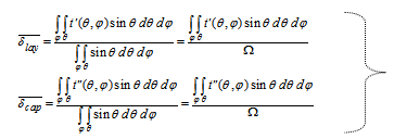 | (8) |
|
 and
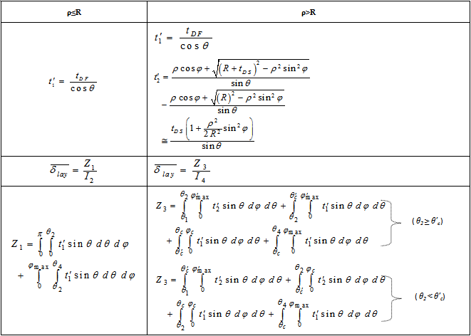
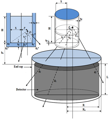
and  are the possible path lengths travelled by the photon within the detector dead layer and end cap material, respectively.Consider the detector has a dead layer by covering its upper surface with thickness
  and its side surface with thickness
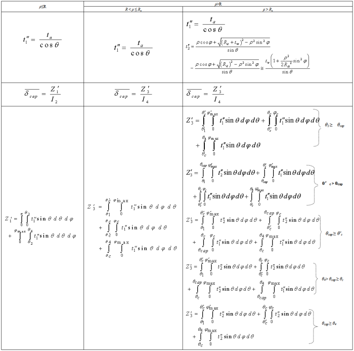
  , (see Figure 1). The possible path lengths and the average path length travelled by the photon within the dead layer for cases (ρ≤R) and (ρ >R) are shown in Table 2, where
  and
and  represents the photon path length through the upper and the side surface of the dead layer respectively.Consider the thickness of upper and side surface of the detector end cap material is
  and tw respectively, as shown in Figure 1. The possible path lengths and the average path length travelled by the photon within the detector end cap material for cases (ρ≤R) and (ρ>R) are shown in Table 3, where
  and
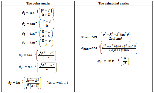
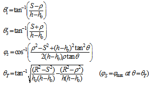
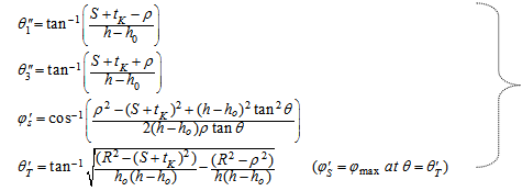
and  represents the photon path length through the upper and the side surface of the detector end cap material, respectively. From Table 4 we observe that, the case in which (ρ>R) has two sub cases which are (R < ρ ≤ Ra) and (ρ > Ra), where Ra is the inner radius of the detector end cap. There is a very important polar angle (θcap ) which must be considered when we study the case in which (ρ > Ra) which is θcap and this is given by:
 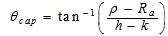 | (9) |
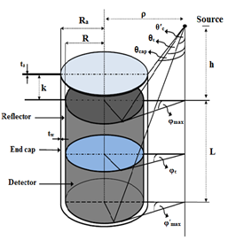 | Figure 1. A diagram of a cylindrical –type detector with a non-axial point source (ρ>R) |
2.2. The Case of a Co-axial Cylindrical Source
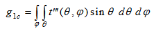
- The efficiency of a cylindrical detector with radius R and height L using a cylindrical source with radius S and height H is given by:
 | (10) |
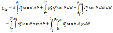
2.2.1. Cylindrical Source with Radius Smaller than or Equal to the Detector’s Radius (S≤R)
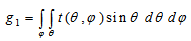
- The intrinsic and geometrical efficiencies are as identified before in Eqs. (2) and (3) respectively, but the average path length
 traveled by the photon through the detector active volume and the solid angle will have new forms due to the geometry of the volumetric source, as shown in Figure 2. The average path length is expressed as:
 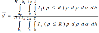 | (11) |
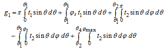
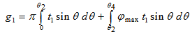
 equation obtained by Abbas et al.(2006) for non axial point source (ρ≤R). α is the angle between the lateral distance ρ and the detector’s major axis. The geometrical efficiency εg is given by:
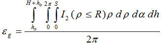 | (12) |
 | (13) |
 is as identified before in Table 2.where
  is as identified before in Table 3.In the case of a co-axial cylindrical source with radius S smaller than the detector radius R, there are two photon possible path lengths to leave the source as follow:ⅰ. To exit from the base
 | (15) |
 | (16) |
 | (17) |
 | (14) |
|
 | Figure 2. The possible cases of the photon path lengths through source – detector system (S≤R) |
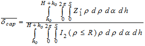
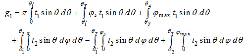
 | (18) |
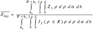
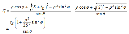
 is the average path length travelled by a photon inside the source and is given by:
 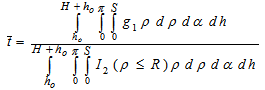 | (19) |
 | (20) |
 | (21) |
 | (22) |
 | (23) |
 is the source container bottom thickness and
  is the source container side thickness, so, there are two photon possible path lengths to exit from the source container as follow:ⅰ. Ⅰ. To exit from the base
 | (24) |
 | (25) |
 | (26) |
 | (27) |
 is the average path length travelled by a photon inside the source container and is expressed as:
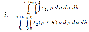 | (28) |
 | (29) |
 | (30) |
 | (31) |
 | (32) |
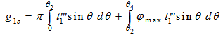
2.2.2. Cylindrical Source with Radius Greater than the Detector’s Radius (S>R)
 | Figure 3. The possible cases of the photon path lengths through source – detector system (S>R) |
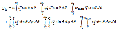
 travelled by the photon through the detector active volume and the solid angle will take new forms due to the geometry of the volumetric source, as shown in Figure 3. The average path length is expressed as:
  | (33) |
 equation obtained by Abbas et al.(2006) for non axial point source. α is the angle between the lateral distance ρ and the detector’s major axis. The geometrical efficiency εg is given by:
 | (34) |
 | (35) |
 and
and  are as identified before in Table 2.
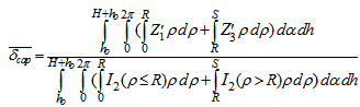 | (36) |
 and
and  are as identified before in Table 3.In the case of a co-axial cylindrical source with radius greater than the radius of the detector, there are two probabilities to be considered; the first probability that the lateral distance of the source is smaller than the detector circular face radius, i.e. ρ ≤ R and the second probability that the lateral distance of the source is greater than the detector circular face radius, i.e. ρ > R and in the two cases, there is only one path to the photon for the way out from the source which is exit from the base and is given by:
 | (37) |
 travelled by a photon inside the source is given by:
 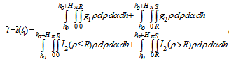 | (38) |
where
 | (39) |
 | (40) |
 is the source container bottom thickness, so, there is only one path of the photon for the way out from the source container which is the exit from the base and is given by:
 | (41) |
 travelled by a photon inside the source container is expressed as:
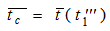 | (42) |
3. Experimental Setup
- The full-energy peak efficiency values are carried out for two NaI (Tl) detectors with resolutions 8.5% and 7.5% at the 662 keV peaks of 137Cs labeled as Det.1 and Det.2 respectively. The manufacturer parameters and the setup values are shown in Table 4.The sources are polypropylene (PP) plastic vials of volumes 25 mL and 400 mL filled with an aqueous solution containing 152Eu radionuclide which emits γ-ray in the energy range from 121 keV to 1408 keV, Table 5 shows sources dimensions. The efficiency measurements are carried out by positioning the sources over the end cap of the detector. In order to minimize the dead time, the activity of the sources is prepared to be (5048 ± 49.98 Bq). The measurements are carried out to obtain statistically significant main peaks in the spectra that are recorded and processed by winTMCA32 software made by ICx Technologies. Measured spectrum which saved as spectrum ORTEC files can be opened by ISO 9001 Genie 2000 data acquisition and analysis software made by Canberra. The acquisition time is high enough to get at least the number of counts 20,000, which make the statistical uncertainties less than 0.5%. The spectra are analyzed with the program using its automatic peak search and peak area calculations, along with changes in the peak fit using the interactive peak fit interface when necessary to reduce the residuals and error in the peak area values. The peak areas, the live time, the run time and the start time for each spectrum are entered in the spreadsheets that are used to perform the calculations necessary to generate the efficiency curves.
| ||||||||||||||||||||
4. Results and Discussion
- The full-energy peak efficiency values for all NaI (Tl) detectors are measured as a function of the photon energy using the following equation
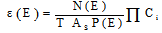 | (43) |
 | (44) |
 | (45) |
 | (46) |
 | (47) |
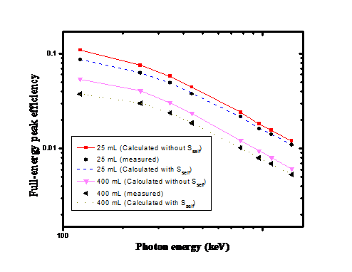 | Figure 4. The full-energy peak efficiencies of a NaI(Tl) detector (Det.1); measured, calculated with Sself and calculated without Sself for different cylindrical sources placed at the end cap of the detector as functions of the photon energy |
| |||||||||||||||||||||||||||||||||||||||||||||||||||||||||||||||||||||||||||||||||||||||||||||||||||
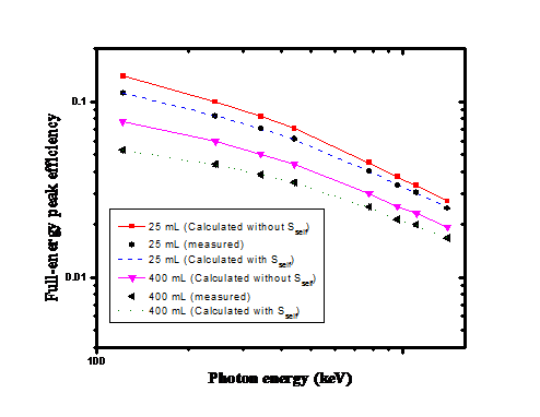 | Figure 5. The full-energy peak efficiencies of a NaI(Tl) detector (Det.2); measured, calculated with Sself and calculated without Sself for different cylindrical sources placed at the end cap of the detector as functions of the photon energy |
5. Conclusions
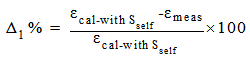
- A direct analytical approach for calculating the full-energy peak efficiency has been derived. In addition, the self attenuation factor of source matrix, the attenuation factors of the source container and the detector housing materials have been calculated. The discrepancies between calculated with Sself and measured full-energy peak efficiency values were found to be less than (1.5%) while, between calculated without Sself and measured full-energy peak efficiency values were found to be less than (32%). The examination of the present results as given in tables and figures reflects the importance of considering the self attenuation factor in studying the efficiency of any detector using volumetric sources.
ACKNOWLEDGEMENTS
- The authors would like to express their sincere thanks to Prof. Dr. Mahmoud. I. Abbas, Faculty of Science, Alexandria University, for the very valuable professional guidance in the area of radiation physics and for his fruitful scientific collaborations on this topic. Dr. Mohamed. S. Badawi would like to introduce a special thanks to The Physikalisch-Technische Bundesanstalt (PTB) in Braunschweig, Berlin, Germany for fruitful help in preparing the homemade volumetric sources.
References
| [1] | Perez, A. A., and Pibida, L., 2004, Performance of CdTe, HpGe and NaI(Tl) detectors for radioactivity measurements. Appl. Radiat. Isot. 60, 41-47. |
| [2] | Vargas, M. J., Timón, A. F., Díaz, N. C., Sánchez, D. P., 2002, Monte Carlo simulation of the self-absorption corrections for natural samples in gamma-ray spectrometry. Appl. Radiat. Isot. 57, 893-898. |
| [3] | Korun, M., 2002, Measurement of the average path length of gamma-rays in samples using scattered radiation. Appl. Radiat. Isot. 56, 77-83. |
| [4] | Lippert, J., 1983, Detector-efficiency calculation based on point-source measurement. Appl. Radiat. Isot. 34, 1097-1103. |
| [5] | Moens, L., and Hoste, J., 1983, Calculation of the peak efficiency of high-purity germanium detectors. Appl. Radiat. Isot. 34, 1085-1095. |
| [6] | Haase, G., Tait, D., Wiechon, A., 1993, Application of new Monte Carl method for determination of summation and self-attenuation corrections in gamma spectrometry. Nucl. Instrum. Methods A336, 206-214. |
| [7] | Sima, O., and Arnold, D., 1996, Self-attenuation and coincidence summing corrections calculated by Monte Carlo simulations for gamma-spectrometric measure- ments with well-type germanium detectors. Appl. Radiat. Isot. 47, 889-893. |
| [8] | Wang, T. K., Mar, W.Y., Ying, T. H., Liao, C. H., Tseng, C. L., 1995, HPGe detector absolute-peak-efficiency calibration by using the ESOLAN program. Appl. Radiat. Isot. 46, 933-944. |
| [9] | Wang, T. K., Mar, W. Y., Ying, T. H., Tseng, C. H., Liao, C. H., Wang, M.Y., 1997, HPGe Detector efficiency calibration for extended cylinder and Marinelli- beaker sources using the ESOLAN program. Appl. Radiat. Isot. 48, 83-95. |
| [10] | Abbas, M. I., 2001, A direct mathematical method to calculate the efficiencies of a parallelepiped detector for an arbitrarily positioned point source. Radiat. Phys. Chem. 60, 3-9. |
| [11] | Abbas, M. I., 2001, Analytical formulae for well-type NaI(Tl) and HPGe detectors efficiency computation. Appl. Radiat. Isot. 55, 245-252. |
| [12] | Abbas, M. I., and Selim, Y. S., 2002, Calculation of relative full-energy peak efficiencies of well-type detectors. Nucl. Instrum. Methods A 480, 651-657. |
| [13] | Selim, Y.S., Abbas, M. I., Fawzy, M. A., 1998, Analytical calculation of the efficiencies of gamma scintillators. Part I: total efficiency of coaxial disk sources. Radiat. Phys. Chem. 53, 589-592. |
| [14] | Selim, Y.S., and Abbas, M. I., 2000, Analytical calculations of gamma scintillators efficiencies. Part II: total efficiency for wide coaxial disk sources. Radiat. Phys. Chem. 58, 15-19. |
| [15] | Abbas, M. I., 2006, HPGe detector absolute full-energy peak efficiency calibration including coincidence correction for circular disc sources. J. Phys. D: Appl. Phys. 39, 3952-3958. |
| [16] | Abbas, M. I., Nafee, S.S., Selim, Y.S., 2006, Calibration of cylindrical detectors using a simplified theoretical approach. Appl. Radiat. Isot. 64, 1057-1064. |
| [17] | Nafee, S. S., and Abbas, M. I., 2008, Calibration of closed-end HPGe detectors using bar (parallelepiped) sources. Nucl. Instrum. Methods A 592, 80-87. |
| [18] | Badawi, M. S., 2010, Ph.D. Dissertation. Alexandria University, Egypt. |