1. Introduction

The detection of ionizing radiation by the scintillation light produced in certain materials is one of the oldest techniques on record. The scintillation process remains one of the most useful methods available for the detection and spectroscopy of a wide assortment of radiations[1].

In 1948, Robert Hofstadter first demonstrated that crystalline sodium iodide, in which a trace of thallium iodide had been added in the melt, produced an exceptionally large scintillation light output compared with the organic materials that had previously received primary attention.This discovery, more than any other single event, ushered in the era of modern scintillation spectrometry of gamma radiation [1].

Most of the inorganic scintillators are crystals of the alkali metals, in particular alkali iodides, that contain a small concentration of an impurity[2]. The alkali halides are good scintillators. In addition to its efficient light yield, sodium iodide doped with thallium NaI(Tl) is almost linear in its energy response[3]. NaI(Tl)’s relatively high density (3.67x10³ kg/m³) and high atomic number combined with the large volume make it a γ-ray detector with very high efficiency[2].

In addition to detecting the presence of radiation, most detectors are also capable of providing some information on the energy of the radiation[4]. A particle energy spectrum is a function giving the distribution of particles in terms of their energies[2].

The energy resolution of a detector (R) is conventionally defined as the full width at half maximum (FWHM) divided by the location of the peak centroid E₀[1] (Fig. 1).

(1)

The energy resolution is thus a dimensionless fraction conventionally expressed as a percentage[1].

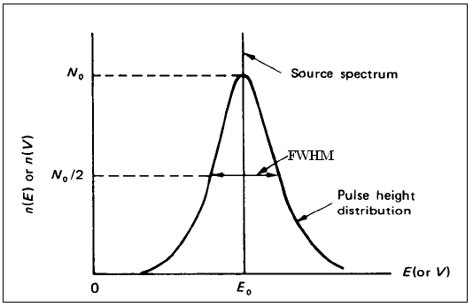
Figure 1. Energy resolution of a detector[2]

The term timing refers to the determination of the time of arrival of a pulse. Timing experiments are used in measurement of the time development of an event (e.g., measurement of the decay of a radioactive species), measurement of true coincident events out of a large group of events, and discrimination of different types of particles based on the different time characteristics of their pulses (pulse shape discrimination)[2].

In a multichannel analyzer (MCA), number of counts versus full scale corresponding to time range of a timing device can be called as a time spectrum. It bears a close relation to the pulse height spectrum. The abscissa, rather than pulse height, is the time interval. The FWHM value of the time distribution is often used as a measure of the overall timing uncertainty in the measurement system and is called the time resolution. The time required for the shaped pulse to reach its maximum amplitude is often called the peaking time[1]. Shaping time can be defined at 61% of the peak value. The peaking time is about 3-5 times greater than the shaping time (Fig. 2)[5].

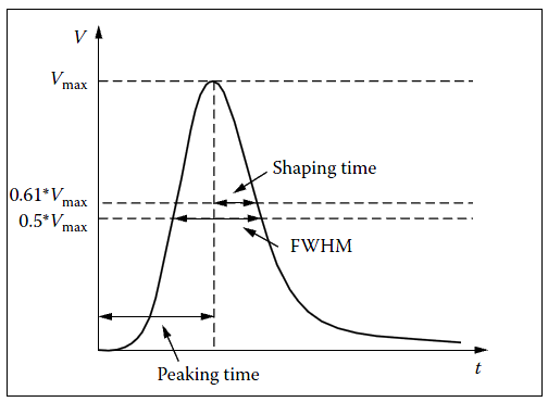
Figure 2. Time spectrum, definitions of shaping and peaking times[5]

Bedwell and Paulus[6] carried out a fast-slow coincidence measurement by using a spectrometer which was consisted of a plastic scintillation detector. A ⁶⁰Co time spectrum was obtained by means of constant fraction timing technique by El-Wahab et al.[7]. Timing resolution of non-delay-line and delay line CFDs was compared for a BGO scintillation detector by Binkley[8]. Pulse shape discrimination (PSD), which is based on the constant fraction timing, was used by Vacik et al.[9] to reduce unwanted background in analyses of solid surfaces by the neutron depth profiling method. Separation of n/γ was achieved by using leading edge timing method in a digital circuit by Jastaniah and Sellin[10]. De Orduna et al.[11] was used the PSD method to reduce background of a BEGe detector. Energy resolution was enhanced by means of pulse rise-time characterization by Troyer et al.[12]. Beta attenuation coefficients of some materials were determined through the constant fraction timing method by Ermis and Celiktas[13]. Kim et al.[14] achieved the separation of n/γ particle by using PSD method.

Gamma energy spectrum of a ¹³⁷Cs radioisotope was obtained by using a NaI(Tl) inorganic scintillation detector in the present work. In order to improve the energy resolution, leading edge and constant fraction timing methods were used. Obtained energy resolution values by using the timing methods were compared with each other. We concluded that the obtained energy resolution value from the constant fraction timing method was better than that of the leading edge timing method.

2. Experiments

Leading edge timing method determines the time of arrival of a pulse with the help of a discriminator. A discriminator threshold is set and the time of arrival of the pulse is determined from the point where the pulse crosses the discriminator threshold[2].

The principle of the leading edge timing method is shown in Fig. 3.

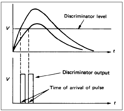
Figure 3. The principle of the leading edge timing method[2]

In constant fraction timing method, the input signal to the constant fraction shaping circuitry is delayed, and a fraction of the undelayed pulse is subtracted from input signal. A bipolar timing pulse is generated, and its zero-crossing is detected and used to produce an output logic pulse[6].

Fig. 4 shows the timing diagram of the constant fraction timing method.

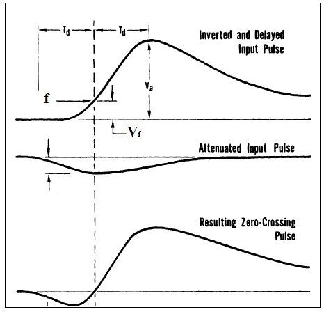
Figure 4. Constant fraction timing method[15]

We used a ¹³⁷Cs radioactive source which has the activity of 5 µCi[16]. The NaI(Tl) scintillation detector manufactured by REXON Inc. has 3 inch diameter and 3 inch length, respectively. The isotope was placed in 4 cm far away from the detector surface, and data acquisition time of 900 s was set during the measurements.

Before the data acquisition, we investigated the effect of the amplifier’s coarse gain level to the noise voltage. For this purpose, we changed the coarse gain of the main amplifier from 10 to 1000 value at constant fine gain. Minimum noise was obtained at the coarse gain value of 50 (Fig. 5). Therefore, the amplifier coarse gain level was fixed to this value during all measurements.

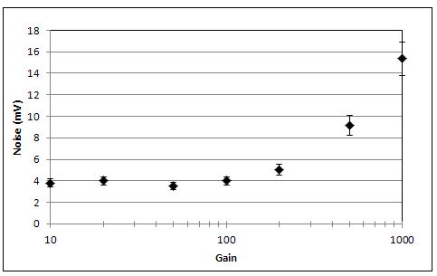
Figure 5. Electronic noise vs. amplifier gain (detector bias= 1000 V)

The time calibration graph was plotted according to variation of peak centroids in time spectrum vs. delay time values of the delay unit as shown in Fig. 6. Time value per channel of the MCA was obtained as the inverse of the slope of time calibration graph, and it was calculated as 12.1±0.1 ps.

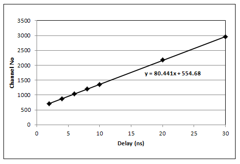
Figure 6. Time calibration graph

In leading edge timing method in the present study, we first obtained the gamma energy spectrum of ¹³⁷Cs and determined the energy resolution of the detector from this spectrum. Then, time spectrum of the isotope was obtained through this method. Finally, energy spectrum was gated by the time spectrum to improve the energy resolution of the detector. Used spectrometer for this process was illustrated in Fig. 7.

In this spectrometer, slow positive signals from the dynode output of the photomultiplier tube (PMT, ORTEC 266) mounted to the detector were sent to a preamplifier (PA, ORTEC 113). Its output was forwarded to a delay line amplifier (DLA, ORTEC 460). Bipolar output of the DLA was split into two branches. Bipolar output was used to avoid the baseline shift. One of these was connected to a multichannel analyzer (MCA, ORTEC Trump 8K) via a delay amplifier (DA, ORTEC 427A) to obtain energy spectrum. The other branch was sent to two timing single channel analyzers (TSCA, ORTEC 420A). One of the TSCAs’ outputs was directly connected to the start input of a time to amplitude converter (TAC, ORTEC 566). The TAC is an electronic device that converts the time difference between two input signals into a voltage pulse between 0 and 10 V. The height of the pulse is proportional to the time difference between the two events[2]. In order to generate time difference between start and stop inputs of the TAC, the other TSCA’s output was first connected to delay unit (D, ORTEC 425A) and then to stop input of the TAC. Time spectrum of the used isotope was obtained by connecting the TAC output to the MCA’s input.

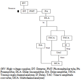
Figure 7. Used spectrometer in leading edge timing method

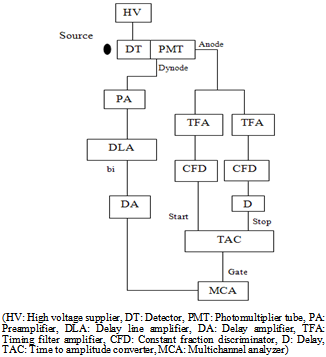
Figure 8. Block diagram of the used spectrometer in constant fraction timing method

Constant fraction timing was used as the second method. The measurements mentioned above were repeated in this method, too. Fig. 8 shows the used spectrometer for this method.

The dynode output of the PMT was sent to the PA. Its output was forwarded to the DLA. Bipolar output of the DLA was connected to the MCA through the DA again. Thus, gamma energy spectrum of ¹³⁷Cs was obtained. Anode output of the PMT was split into two branches. These branches were forwarded to two timing filter amplifiers (TFA, ORTEC 454). The TFA provides additional gain before the timing discriminator. Integration in the TFA can be used to reduce high frequency noise[17]. Outputs of the TFAs were connected to two constant fraction discriminators (CFD, ORTEC 463). The CFD module triggers at a fixed fraction of the input signal amplitude to produce a logic marker[9]. One of the CFDs’ output was forwarded directly to start input of the TAC. In order to generate time difference between start and stop inputs of the TAC, the other CFD’s output was connected to the delay (D) then forwarded to TAC’s stop input. Time spectrum of the isotope can be obtained from this part of the spectrometer.

The integration time constant of the amplifier was set to 0.04 µs. This value was chosen to provide the equality between shaping and peaking times mentioned above.

TSCA, CFD, DLA and TAC output signal shapes are shown in Figs. 9 and 10.

In order to investigate the effect of CFD’s threshold level to time resolution, we changed the start CFD’s threshold level from 0.08 to 4.00 V, and we found optimum threshold level as 0.08 V for best time resolution as can be seen in Fig. 11.

We checked whether or not the delay time was effective on the time resolution, also. For this purpose, we recorded the time resolutions versus delay time values. We plotted these data as shown in Fig. 12. According to this graph, optimum time resolution was determined at the delay time of 2 ns. Therefore, all measurements in constant-fraction timing method were carried out at this delay time.

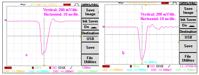
Figure 9. (a) TSCA (b) CFD output signal shapes

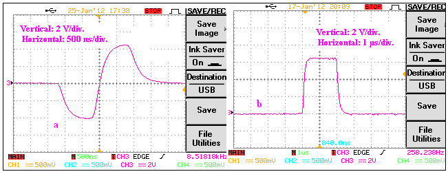
Figure 10. (a) DLA bipolar (b) TAC output signal shapes

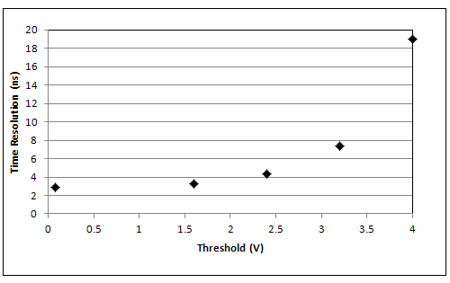
Figure 11. Time resolution vs. CFD threshold

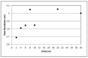
Figure 12. Time resolution vs. delay

3. Results and Discussions

Background energy spectrum was recorded to consider its effect to the obtained energy spectra. Background energy spectrum is given in Fig. 13. Since the number of counts is quite low in comparison with the source energy spectrum, it can be deduced from this background spectrum that the background is not effective on the obtained energy spectra.

Figure 13. Background energy spectrum

Obtained time spectrum through the leading edge timing method of the isotope can be seen in Fig. 14. Time resolution value from this spectrum was found as 1.67 ns.

Fig. 15(a) shows the only gamma ray energy spectrum of ¹³⁷Cs with the photopeak energy resolution of 8.77%. Coincident energy spectrum, i.e. gamma energy spectrum in Fig. 15(a) gated by the time spectrum in Fig. 14, is shown in Fig. 15(b). The photopeak energy resolution of 8.46% was calculated in this spectrum. Energy (a) and the coincident (b) energy spectra of the isotope via leading edge timing method can be compared in Fig. 15.

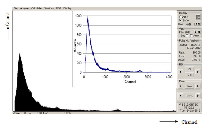
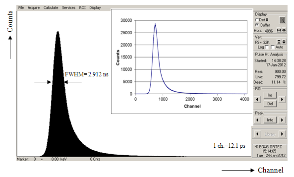
Figure 14. Time spectrum of 137Cs by means of leading edge timing method

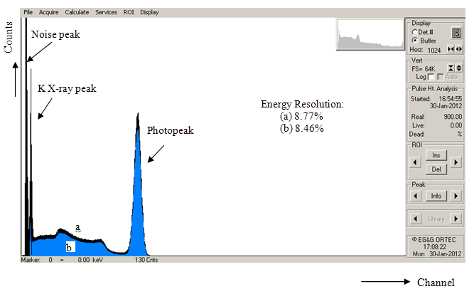
Figure 15. Comparison of the energy spectra before (a) (black) and after (b) (blue) leading edge timing method

Gross count rates under the photopeaks in the energy (Fig. 15a) and the coincident (Fig. 15b) spectra were calculated as 990.87 and 864.17 s^-1, respectively in this timing method.

In leading edge timing method, the shaping and peaking times were found through the DLA output as 280 and 900 ns, respectively. It can be seen from this result that the peaking time is about three times greater than the shaping time as expected.

In constant fraction timing method, the shaping and peaking times were determined from both the TFA and the DLA outputs to check the relation between these time values. The shaping and peaking times were found as 70 and 200 ns, respectively in the TFA output signal. These time values were obtained as 280 ns and 1 µs, respectively for the DLA output signal. The peaking times for this timing method was found again about three times greater than the shaping times.

After application of the constant fraction timing method, obtained time spectrum of the isotope was given in Fig. 16. Time resolution of 2.912 ns was calculated from this spectrum.

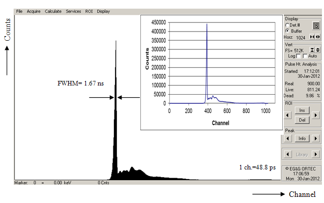
Figure 16. Time spectrum of 137Cs by means of constant fraction timing method

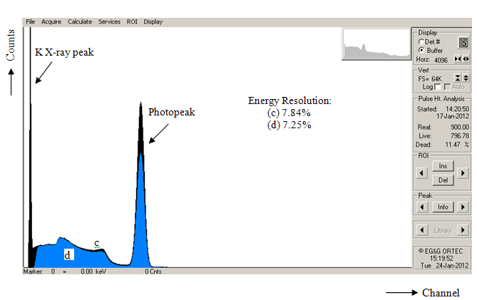
Figure 17. Comparison of energy spectra before (c) (black) and after (d) (blue) constant fraction timing method

In Fig. 17(c), the gamma ray energy spectrum of the isotope is shown again to deal with the constant fraction timing method. The photopeak energy resolution from this spectrum was calculated as 7.84%.

To improve the energy resolution value, energy spectrum of the isotope was gated by constant fraction timing signal. Coincident energy spectrum with the photopeak energy resolution of 7.25% is shown in Fig. 17(d). Comparison of the energy spectra before and after constant fraction timing method can be seen in this figure.

Horizontal and vertical axes in the figures above correspond to the number of channels and counts, respectively.

Photopeak gross count rates for energy and coincidence spectra were found so as to be 4,580 and 3,180 s^-1, respectively in the measurements of constant fraction timing method.

The photopeak gross areas for both leading edge (864.17 s^-1) and constant fraction timing method (3,180 s^-1) were less than 5,000 s^-1 which means that these values point out generally slow count rates in the measurement[18]. In high count rates (above 5,000 s^-1), the MCA exhibits high dead time percentage (over than 30-40%), leading to pulse pile-up and spectrum distortions[1, 4]. As can be seen in the energy spectra above, the recorded dead time values by the MCA were below the reported level. We can conclude from this result that the obtained spectra have no pulse pile-up effect and distortion, increasing their reliabilities.

Dynamic range can be defined as the ratio between the input signal amplitude and the noise threshold[5]. If the dynamic range is narrow, the count rate in the MCA becomes low. The leading edge timing method gives the better results at low dynamic ranges[15, 18, 19]. Therefore, we used low count rate (864.17 s^-1) in this timing method. Since the constant fraction timing method gives the better results at relatively high count rates[15, 18, 19], the count rate in the second method was fixed to higher (3,180 s^-1) than that of the leading edge timing.

Since time resolution has affected from the change of the CFD threshold level[6, 17], the variation of the time resolution vs. the threshold level of the start CFD from 0.08 to 4.00 V was observed to obtain best resolution value. Optimum threshold level was determined as 0.08 V as can be seen in Fig. 11. Therefore, the threshold levels of the CFDs were set to this value and never changed during all measurements.

Investigation of the minimum noise voltage versus the optimum amplifier coarse gain value showed that coarse gain level of the amplifier was effective on the spectrometer performance.

The spectrometer energy resolution is normally affected from the electronic noise[3]. Therefore, the noise peak in low energy region was discriminated in the final energy spectra through both timing methods.

4. Conclusions

We aimed to improve the energy resolution of ¹³⁷Cs energy spectrum of a NaI(Tl) inorganic scintillation detector in this study. Leading edge and constant fraction timing methods were used for this purpose. Obtained results showed that both methods can be used for the energy resolution enhancement of a NaI(Tl) scintillation detector.

In the first timing method, energy resolution of the detector was calculated as 8.77% without any timing application. After application of the leading edge timing method, this value was decreased to 8.46% which corresponds to an improvement of 3.5%. In the second section of the work, the energy resolution value with constant fraction timing method was calculated as 7.25% while the value without constant fraction timing method was found as 7.84% which means that an energy resolution enhancement of 7.5% was obtained. It can be concluded from both results that the leading edge and the constant fraction timing methods can be used to improve the energy resolution of a NaI(Tl) scintillation detector. However, better energy resolution value was obtained by using constant fraction timing method than that of the leading edge method as indicated in various studies[15, 17].

As a consequence of the obtained results, it can be concluded that these analog timing methods can be easily used for the energy resolution enhancement of any type of inorganic scintillation detector.

ACKNOWLEDGEMENTS

This work was supported by TUBITAK, the Scientific and Technical Research Council of TURKEY under project numbers 197T087 and 111T571, and by EBILTEM, Center of Science and Technology, Ege University under project no. 99 BIL 001, and finally Scientific Research Foundation of Ege University under project no. 11 FEN 085.

References

[1]  G.F. Knoll, ‘Radiation Detection and Measurements’, John Wiley & Sons. Inc, New York, 2000.
[2]  N. Tsoulfanidis, ‘Measurements and Detection Radiation’, Taylor & Francis, USA, 1995.
[3]  J.E. Turner, ‘Atoms, Radiation and Radiation Protection’, Wiley-VCH Verlag GmbH&Co. KGaA, Weinheim, 2007.
[4]  R.W. Leo, ‘Techniques for Nuclear and Particle Physics Experiments’, Springer–Verlag Berlin Heidelberg, Germany, 1987.
[5]  S.P. Bönisch, ‘Electronics for Radiation Detection’, CRC Press, U.S., 2011.
[6]  M.O. Bedwell and T.J. Paulus, ‘A Constant Fraction Differential Discriminator for Use in Fast Timing Coincidence Systems’, IEEE Trans. Nucl. Sci. 26, 422-427, 1979.
[7]  M.A. El-Wahab, A. El-Arabi, M.H. Battrawi, ‘Constant Fraction Timing With Scintillation Detectors’, IEEE Trans. Nucl. Sci. 36, 401-406, 1989.
[8]  D.M. Binkley, ‘Performance of Non-delay-line Constant - fraction Discriminator Timing Circuit’, IEEE Trans. Nucl. Sci. 41, 1169-1175, 1994.
[9]  J. Vacik, J. Cernava, V. Hnatowicz, V. Havranek, J. Hoffmann, S. Posta, D. Fink, R. Klett, ‘Pulse-shape Discrimination in Neutron Depth Profiling Technique’, Nucl. Instrum. Meth. B 142, 397-401, 1998.
[10]  S.D. Jastaniah and P.J. Sellin, ‘Digital Techniques for n/γ Pulse Shape Siscrimination and Capture-gated Neutron Spectroscopy Using Liquid Scintillators’, Nucl. Instrum. Meth. A 517, 202-210, 2004.
[11]  R.G. De Orduna, M. Hult, E. Andreotti, D. Budjas, S. Schönert, M. Misiaszek, M., ‘Pulse Shape Analysis to Reduce The Background of BEGe Detectrors’, J. Radioanal. Nucl. Chem. 286, 477-482, 2010.
[12]  G.L. Troyer, B.D. Keele, G.C. Tepper, ‘Pulse Rise-time Characterization of a High Pressure Xenon Gamma Detector for Use in Resolution Enhancement’, J. Radioanal. Nucl. Chem. 248, 267-281, 2001.
[13]  E.E. Ermis and C. Celiktas, ‘Determination of Beta Attenuation Coefficients by Means of Timing Method’, Ann. Nucl. Energy 41, 115-118, 2012.
[14]  W.S. Kim, H.S. Kim, K.H. Kim, Y.U. Kim, K.H. Kim, ‘Gamma-ray Pulse-height Spectrum of 241Am –Be Source by Li-BC501 (n-γ) Spectrometer System’, J. Radioanal. Nucl. Chem. 215, 257-261, 1997.
[15]  R. Nutt, D.A. Gedcke, C.W. Williams, ‘A Comparison of Constant Fraction and Leading Edge Timing with NaI(Tl) Scintillators’, IEEE Trans. Nucl. Sci. 17, 299-306, 1970.
[16]  http://www.matpack.de/Info/Nuclear/Nuclids/nuclids9.html Accessed 23 March 2012.
[17]  M.O. Bedwell and T.J. Paulus, ‘A New Constant Fraction Timing System With Improvement Time Derivation Characteristics’, IEEE Trans. Nucl. Sci. 23, 234-243, 1976.
[18]  T.J. Paulus, ‘Timing Electronics and Fast Timing Methods With Scintillation Detectors’, IEEE Trans. Nucl. Sci. 32, 1242-1249, 1985.
[19]  M. Moszynski and B. Bengston, ‘Status of Timing With Scintillation Detectors’, Nucl. Instrum. Meth. 158, 1-31, 1979.