Ahmed. M. El-Khatib 1, Mohamed. S. Badawi 1, Mohamed. A. Elzaher 2, Abouzeid. A. Thabet 2
1Physics Department, Faculty of Science, Alexandria University, 21511 Alexandria, Egypt
2Department of Basic and Applied Sciences, Faculty of Engineering, Arab Academy for Science, Technology and Maritime Transport, Alexandria, Egypt
Correspondence to: Mohamed. S. Badawi , Physics Department, Faculty of Science, Alexandria University, 21511 Alexandria, Egypt.
| Email: |  |
Copyright © 2012 Scientific & Academic Publishing. All Rights Reserved.
Abstract
In this work the Full-Energy Peak Efficiency (FEPE) of NaI(Tl) - scintillation detectors (5.08x5.08 cm2and 7.62x7.62 cm2) values are calculated for coaxial cylindrical sources with radii greater than the detectors faces radii. This was calculated by the effective solid angle method, taking into account the source self-attenuation effect. In the experiments the gamma sources that contain several radionuclides covering the energy range from 59.52 to 1408.01 keV were used. By comparison, it was found that the theoretical and the experimental FEPE values are in a good agreement.
Keywords:
NaI (Tl) Detector, Full-Energy Peak Efficiency, Efficiency Transfer, Effective Solid Angle
1. Introduction
Determining the experimental detector efficiency is an inflexible and a time consuming process, this is due to its scientific and industrial importance. The interest for computational techniques based on different principles, models, and assumptions increased during the last years. One of these computational techniques is the efficiency transfer principle in which the computation of the detector efficiency for various geometrical conditions is derived from the known efficiency for reference source-detector geometry. The main advantage of the efficiency transfer approach with a point calibration source located at a sufficient distance from the detector is that one may neglect the coincidence summing effects and obtain a coincidence free efficiency curve,[1]. The efficiency transfer method is particularly useful due to its insensitivity to the inaccuracy of the input data, such as the uncertainty of the detector characterization[2,3]. The presented approach is based on the direct mathematical method reported by Selim and Abbas[4-11]. It was used successfully before to calibrate point, plane, and volumetric sources with cylindrical, well-type, parallelepiped, and 4π NaI(Tl) detectors.The changes in efficiency under measurement conditions differ from those of calibration. This can be determined by the basis of variation of the geometrical parameters of the source-detector arrangement. By calculation, it is possible todetermine the efficiency corresponding to non-point samples and/or for different distances. The efficiency of the basic case corresponding to the calibration with known efficiency for a point source located at position Pο and at energy E can be expressed as: | (1) |
where  represents the intrinsic efficiency of the detector for energy E and
  is the effective solid angle subtended by point Pο and the active surface of the detector. This geometrical factor must include absorbing factors, taking into account the attenuation effects in the materials between the source and the active part of the crystal[12]. Similarly, for a point source located at a different distance P the efficiency can be written as:
  | (2) |
So we can establish the basic relationship which makes it possible to express the efficiency as a function of the reference efficiency, known at the same energy E as in equation (3):  | (3) |
In general by knowing the source-detector geometry, we can compute the detector efficiency for different shapes using the principle of efficiency transfer by computing the relevant solid angle and absorbing factors[13].
2. Mathematical Treatment
Selim and co-workers used the spherical coordinate system to derive the direct analytical elliptic integrals and to calculate the detector efficiencies (total and full-energy peak) for any source-detector configuration,[14]. The solid angle (Ω) subtended by the detector at the source point is introduced in[8] and it is defined as: | (4) |
while the effective solid angle is defined as: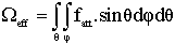 | (5) |
where fatt is the factor that determines the photon attenuation by all absorbers between source and detector, it is expressed as: | (6) |
where μi is the attenuation coefficient of the ith absorber for a gamma-ray photon with energy Eγ and δi is the average gamma photon path length through the ith absorber.The location of an arbitrarily positioned axial point source is specified by the source-detector distance (h) shown in figure (1), and the polar (θ) and the azimuth (φ) angles which are at the point of entrance of the considered surface defined by the direction of the incidence of a gamma-ray photon.The polar angles can be expressed as, (Abbas et al., 2007).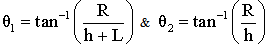 | (7) |
Therefore the effective solid angle can be expressed as: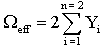 | (8) |
where: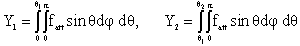 | (9) |
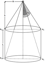 | Figure 1. An axial point source with Cylindrical Detector |
The volumetric source can be treated as group of point sources which are uniformly distributed; each point source has an effective solid angle  ,[15] as shown in equation (10).
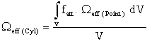 | (10) |
To calculate the effective solid angle of a detector using a radioactive cylindrical source of dimensions larger than the detector, choose an arbitrary element of volume dV at lateral distance ρ from the detector axis that makes an angle α with the detector’s major axis h. Where h is the source-detector separation, this element of volume can be expressed in the polar coordinates by: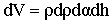 Therefore, equation (10) will be:
 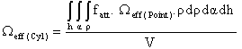 | (11) |
In volumetric source, not all the emitted photons from the source exit from it, but part of them is absorbed in the source itself, which affects the effective solid angle calculations. The factor concerning this effect is called the self-absorption factor Sf which is given by:[15]. | (12) |
where μs is the source attenuation coefficient and ds is the distance traveled by the emitted photon inside the source as shown in figure (2). ds was found to be a function of the polar and azimuthal angles (θ, φ) inside the source itself and it is given by: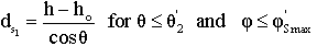 | (13) |
Therefore, the source polar and azimuthal angles can be given as equations (14) and (15), respectively:[15]. 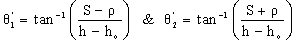 | (14) |
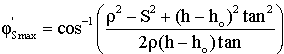 | (15) |
Where θ'1 and θ'2 are the extreme polar angles of the source, φ'Smax is the maximum azimuthal angle for the photon to exit the source, and ho is the source-detector separation.So equation (11) can be written as follows: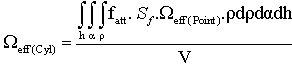 | (16) |
Thus, the effective solid angle of a cylindrical detector in case of a cylindrical source of radius (S≥R) and height H can be expressed by:  | (17) |
 | Figure 2. Cylindrical source and detector configuration (S≥R) |
So the detector efficiency using cylindrical sources can be calculated by the efficiency transfer principle as follow:  | (18) |
3. Experimental Setup
In this work two NaI (Tl) scintillation detectors are used. The (5.08x5.08 cm2) detector (D1) with resolution 8.5% and (7.62x7.62 cm2) detector (D2) with resolution 7.5%, both of them are specified at 661 keV. The details of these detectors setup parameters with acquisition electronics specifications supported by the serial and model number are listed in Table 1. The FEPE has been measured using two types of radioactive sources. The point sources for first one are 241Am, 133Ba, 152Eu, 137Cs, and 60Co.T point sources were purchased from the Physikalisch-Technische Bundesanstalt (PTB) in Braunschweig and Berlin. The certificates show the sources activities and their uncertainties for PTB sources which are listed in Table 2. The data sheet states the values of half-life photon energies and photon emission probabilities per decay for all radionuclides used in the calibration process are listed in table (3), which is available at the National Nuclear Data Center Web Page or on the IAEA website.| Table 1. Detectors setup parameters with acquisition electronics specifications for Detector (D1) and Detector (D2) |
| | Items | Detector (D1) | Detector (D2) | | Manufacturer | Canberra | Canberra | | Serial Number | 09L 654 | 09L 652 | | Detector Model | 802 | 802 | | Type | cylindrical | cylindrical | | Mounting | vertical | vertical | | Resolution (FWHM) at 661 kev | 7.5% | 8.5% | | Cathode to Anode voltage | +1100 V dc | +1100 V dc | | Dynode to Dynode | +80 V dc | +80 V dc | | Cathode to Dynode | +150 V dc | +150 V dc | | Tube Base | Model 2007 | Model 2007 | | Shaping Mode | Gaussian | Gaussian | | Detector Type | NaI(Tl) | NaI(Tl) | | Crystal Diameter (mm) | 50.8 | 76.2 | | Crystal Length (mm) | 50.8 | 76.2 | | Top cover Thickness(mm) | Al (0.5) | Al (0.5) | | Side cover Thickness(mm) | Al (0.5) | Al (0.5) | | Reflector – Oxide (mm) | 2.5 | 2.5 | | Weight (Kg) | 0.77 | 1.8 | | Outer Diameter(mm) | 57.2 | 80.9 | | Outer Length(mm) | 53.9 | 79.4 | | Crystal Volume in (cm3) | 103.004 | 347.639 |
|
|
| Table 2. PTB point sources activities and their uncertainties |
| | PTB- Nuclide | Activity (KBq) | Reference Date00:00 Hr | Uncertainty (KBq) | | 241Am | 259.0 | 1.June 2009 | ±2.6 | | 133Ba | 275.3 | ±2.8 | | 152Eu | 290.0 | ±4.0 | | 137Cs | 385.0 | ±4.0 | | 60Co | 212.1 | ±1.5 |
|
|
The calibration process was done by using the (PTB) point sources. The homemade Plexiglas holder is used to measure these sources at seven different axial distances starting from 20 cm till 50 cm with 5 cm step from the detectors surface. The holder is placed directly on the detector entrance window as an absorber. In most cases the accompanying x-ray was soft enough to be absorbed completely before entering the detector. To avoid the effect of β- and x- rays and to protect the detector heads, therefore, there is no correction was made for x-gamma coincidences. The source-detector separations start from 20 cm to neglect the coincidence summing correction.The second type of source is the 500 ml Polypropylene volumetric source made by Nalgene Lab-ware, its catalog number is (NG-2118), the size code is (16) filled with 200, 300, and 400 ml 152Eu solution of known activity, the details of the prepared sources are tabulated in table (4) | Figure 3. Homemade Plexiglas Holder parts Drawing |
| Table 3. Half lives, photon energies and photon emission probabilities per decay for the all radionuclides used in this work |
| | PTB-Nuclide | Energy (Kev) | Emission Probability % | Half Life (Days) | | 241Am | 59.52 | 35.9 | 157861.05 | | 133Ba | 80.99 | 34.1 | 3847.91 | | 152Eu | 121.78 | 28.4 | 4943.29 | | 244.69 | 7.49 | | 344.28 | 26.6 | | 778.9 | 12.96 | | 964.13 | 14.0 | | 1408.01 | 20.87 | | 137Cs | 661.66 | 85.21 | 11004.98 | | 60Co | 1173.23 | 99.9 | 1925.31 | | 1332.5 | 99.982 |
|
|
| Table 4. Prepared sources (homemade) details |
| | Volume | Nuclide | Activity (KBq) | Reference Date 00:00 Hr | Uncertainty (KBq) | | V1 (200 ml) | 152Eu | 5 | 1.Jan 2010 | ±4.0 | | V2 (300 ml) | | V3(400 ml) |
|
|
As an example if the spectrum was recorded as P4D1 where P refers to the source type (point) measured on detector (D1) at distance number (4), hence h = 20 cm.The volumetric sources (vials) were measured on a 0.1 cm thick Plexiglas cover and placed directly on the detector end-cap. These measurements were done using two cylindrical detectors with numbers (D1 and D2). The source was placed on the detector end-cap with the center of the source centered on the end-cap. The spectra was recorded as V1D2, where V1 is the volume (V1) measured on detector (D2). The angular correlation effects can be neglected for the low source-to-detector distance,[16]. The spectrum acquired with winTMCA32 software is made by ICx Technologies. It was analyzed with Genie 2000 data acquisition and analysis software. It was made by Canberra using the automatic peak search and the peak area calculations, along with changes in the peak fit using the interactive peak fit interface when necessary to reduce the residuals and errors in the peak area values. The live time, the run time, and the start time for each spectrum are entered in the spread sheets. Those sheets were used to perform the calculations necessary to generate the experimental FEPE curves with their associated uncertainties as a function of the photon energy for all calibration sources detectors listed in tables (4).The Efficiency Transfer for Nuclide Activity measurements (ETNA) program and the Efficiency Transfer Theoretical Method (ETTM) used to convert the FEPE curve from point sources at position (P4, P5, P6, P7, P8, P9, and P10) to the FEPE of other geometries which represented in V1, V2, and V3. These calculations extended for two cylindrical NaI(Tl) detectors (D1, and D2).
4. Results and Discussions
This section shows a comparison between the theoretical and the experimental work of the efficiency transfer method (ETTM). The experimental work was held at Younis. S. Selim laboratory for Radiation Physics, Faculty of Science, Alexandria University. This laboratory uses several coaxial NaI (Tl) scintillation detectors (5.08x5.08 cm2 and 7.62x7.62 cm2) which are used in the presented work. The detectors were calibrated by measuring the low activity point sources, previously described. The theoretical FEPE can be obtained as given in equation (18).Another method of calibration is by using ETNA program developed in the Laboratoire National Henri Becquerel (BNM/LNHB) CEA/Saclay, France by (Marie Christine Lepy[17].The percentage error between the measured and the calculated efficiencies is given by:  | (19) |
where εcal and εmeas are the calculated and experimentally measured efficiencies, respectively. The measured efficiency values as a function of the photon energy ε(E) for all NaI Scintillation detectors were calculated by:  | (20) |
where N(E) is the number of counts in the full-energy peak and it can be obtained using Genie 2000 software, T is the measuring time (in second), P(E) is the photon emission probability at energy E, AS is the radionuclide activity, and Ci, are the correction factors due to dead time and radionuclide decay. For the measurements of the low activity sources, the dead time was always less than 3%, so the corresponding factor was obtained simply using ADC live time. The statistical uncertainties of the net peak areas were smaller than 1.0 %. Since the acquisition time was long enough to get the number of counts which was at least 10,000 counts. Therefore, the background subtraction was done. The decay correction Cd for the calibration source from the reference time to the run time was given by: | (21) |
where λ is the decay constant and ΔT is the time interval over which the source decays corresponding to the run time. The main source of uncertainty in the efficiency calculations was the uncertainties of the activities of the standard source solutions. The coincidence summing effects were negligible in the reference measurement geometries.The uncertainty in the FEPE σε was given by:  | (22) |
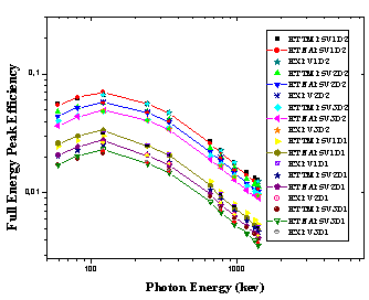
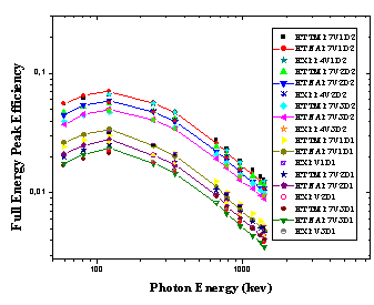
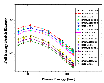
where σA, σP, and σN, are the uncertainties associated with the quantities AS, P(E), and N(E), respectively, assuming that the only correction made is due to the source activity decay. In order to study the effect of the detector volume and the source-to-detector distance on the FEPE of NaI (Tl) detectors (D1 and D2) and of volumes (V1, V2, and V3), the measured efficiency for different sources detector arrangement were compared. Figure (4-17) show that the efficiency is increasing by decreasing the source volume (all sources have the same radius, vessel, and carrier solution, only the height of the source is different). The self-attenuation effect increased by increasing the carrier solution as we know when the attenuation factors increase then the number of photons reach the detector decrease. Moreover, the efficiency is increased with increasing the detector’s volume, where the crystal should be long enough to have reasonable efficiency for the highest energy gamma-rays of interest. This is due to the change in solid angle and increasing the chance of various interactions of photon with the detector material as a result of increasing the pass length in the crystal of larger volume.The efficiency of the detectors is high at low source energies (absorption coefficient is very high) and decreases as the energy increases (fall off in the absorption coefficient). This is due to the fact that the photoelectric is dominant below 100 keV, which means in other words that it is higher for the bigger detector than the smaller one and it is higher for lower source energy than higher source energy. This is because of the dominance of the photoelectric at lower source energies.The presented work provides a great understanding to several aspects of gamma-ray spectroscopy and will provide us with useful tools (ETTM) for efficiency calculation for co-axial detectors. This method constitutes a good approach for the efficiency computation for laboratory routine measurements and can save time in avoiding experimental calibration for different position geometries. Where the values of the efficiency calculations using (ETTM) was compared with the measured ones and the results from ETNA program.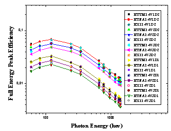 | Figure 4. ETNA and ETTM efficiency results for conversion from point sources at (P4) to (V1, V2, and V3) using detectors (D1, and D2), and the measured ones for (V1D2, V2D2, V3D2, V1D1, V2D1, and V3D1) arrangement |
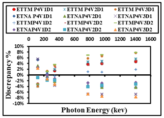 | Figure 5. The difference percentage (Δ%) between ETNA, ETTM (P4V1,P4V2, and P4V3) results and its corresponding experimental values of detectors (D1, and D2) calculated as a function of the photon energy |
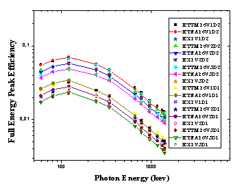
 | Figure 6. ETNA and ETTM efficiency results for conversion from point sources at (P5) to (V1, V2, and V3) using detectors (D1, and D2), and the measured ones for (V1D2, V2D2, V3D2, V1D1, V2D1, and V3D1) arrangement |
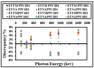 | Figure 7. The difference percentage (Δ%) between ETNA, ETTM (P5V1,P5V2, and P5V3) results and its corresponding experimental values of detectors (D1, and D2) calculated as a function of the photon energy |
 | Figure 8. ETNA and ETTM efficiency results for conversion from point sources at (P6) to (V1, V2, and V3) using detectors (D1, and D2), and the measured ones for (V1D2, V2D2, V3D2, V1D1, V2D1, and V3D1) arrangement |
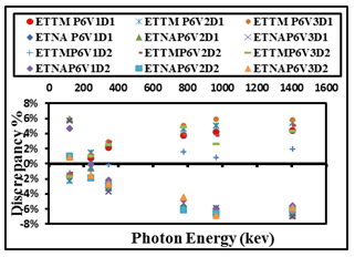 | Figure 9. The difference percentage (Δ%) between ETNA, ETTM (P6V1,P6V2, and P6V3) results and its corresponding experimental values of detectors (D1, and D2) calculated as a function of the photon energy |
 | Figure 10. ETNA and ETTM efficiency results for conversion from Point sources at (P7) to (V1, V2, and V3) using detectors (D1, and D2), and the measured ones for (V1D2, V2D2, V3D2, V1D1, V2D1, and V3D1) arrangement |
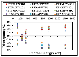 | Figure 11. The difference percentage (Δ%) between ETNA, ETTM (P7V1, P7V2, and P7V3) results and its corresponding experimental values of detectors (D1, and D2) calculated as a function of the photon energy |
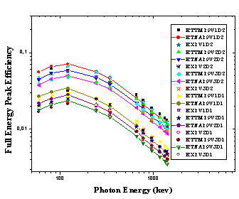
 | Figure 12. ETNA and ETTM efficiency results for conversion from point sources at (P8) to (V1, V2, and V3) using detectors (D1, and D2), and the measured ones for (V1D2, V2D2, V3D2, V1D1, V2D1, and V3D1) arrangement |
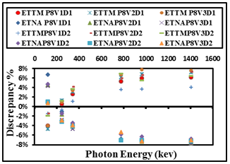 | Figure 13. The difference percentage (Δ%) between ETNA, ETTM (P8V1, P8V2, and P8V3) results and its corresponding experimental values of detectors (D1, and D2) calculated as a function of the photon energy |
 | Figure 14. ETNA and ETTM efficiency results for conversion from point sources at (P9) to (V1, V2, and V3) using detectors (D1, and D2), and the measured ones for (V1D2, V2D2, V3D2, V1D1, V2D1, and V3D1) arrangement |
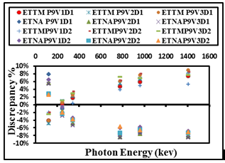 | Figure 15. The difference percentage (Δ%) between ETNA, ETTM (P9V1, P9V2, and P9V3) results and its corresponding experimental values of detectors (D1, and D2) calculated as a function of the photon energy |
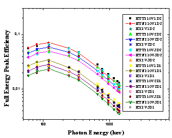 | Figure 16. ETNA and ETTM efficiency results for conversion from point sources at (P10) to (V1, V2, and V3) using detectors (D1, and D2), and the measured ones for (V1D2, V2D2, V3D2, V1D1, V2D1, and V3D1) arrangement |
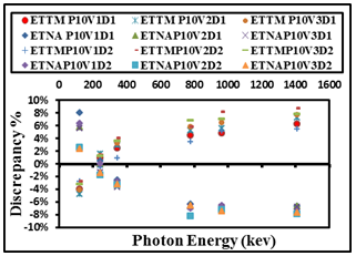 | Figure 17. The difference percentage (Δ%) between ETNA, ETTM (P10V1, P10V2, and P10V3) results and its corresponding experimental values of detectors (D1, and D2) calculated as a function of the photon energy |
5. Conclusions
This work led to a simple (ETTM) to evaluate the FEPE over a wide energy range, which deal with different detector types for isotropic axial point sources, and axial cylindrical sources. Accordingly the present approach shows great possibilities to calibrate the detectors through the determination of the FEPE curve even in those cases when no standard source is available, which is considered as the final goal of this work. The discrepancies in general for all the measurements were found to be less (10%) in case of ETNA program and our (ETTM) expressions and experimental values at all energy region.
ACKNOWLEDGMENTS
The authors would like to express their sincere thanks to Prof. Mahmoud. I. Abbas, Faculty of Science, Alexandria University, for the very valuable professional guidance in the area of radiation physics and for his fruitful scientific collaborations on this topic.Dr. Mohamed. S. Badawi would like to introduce a special thanks to The Physikalisch-Technische Bundesanstalt (PTB) in Braunschweig, Berlin, Germany for their fruitful help in preparing the homemade volumetric sources.
References
| [1] | Vidmar T, Vodenik B, Necemer M: Efficiency transfer between extended sources” Applied Radiation and Isotopes 2010; 68:2352–2354. |
| [2] | Le´py MC, Altzitzoglou T, Arnold D, Bronson F, Capote Noy R, Décombaz M, et al. Intercomparison of efficiency transfer software for gamma-ray spectrometry Applied Radiation and Isotopes 2001; 55(4):493–503. |
| [3] | Vidmar T, Aubineau-Laniece I, Anagnostakis MJ, Arnold D, Brettner-Messler R, Budjas, Aubineau LI D, et al. An intercomparison of Monte Carlo codes used in gamma-ray spectrometry. Applied Radiation and Isotopes 2008; 66(6–7):764–768. |
| [4] | Abbas MI, HPGe detector photopeak efficiency calculation including self-absorption and coincidence corrections for Marinelli beaker sources using compact analytical expressions Applied Radiation and Isotopes 2001;54:761-768. |
| [5] | Abbas MI and Selim YS, Calculation of relative full-energy peak efficiencies of well-type detectors Nucl. Instrum. Methods Phys. Res. 2002; A, 480(2-3):651-657. |
| [6] | Abbas MI, Nafee SS, Selim YS, A simple mathematical method to determine the efficiencies of log-conical detectors Radiation Physics and Chemistry 2006;(75):729-736. |
| [7] | Mahmoud I. Abbas,. ”HPGe detector absolute full-energy peak efficiency calibration including coincidence correction for circular disc sources” J. Phys. D: Appl. Phys. 2006;39 (3952–3958). |
| [8] | L. Pibida, S.S. Nafee, M. Unterweger, M.M: Hammond, L. Karam and M. I. Abbas: Calibration of HPGe gamma-ray detectors for measurement of radioactive noble gas sources Applied Radiation and Isotopes Journal 2007;65:225-233 |
| [9] | Abbas, M.I., 2007. Direct mathematical method for calculating full-energy peak efficiency and coincidence corrections of HPGe detectors for extended sources. Nucl. Instrum. Methods B, 256: 554-557. |
| [10] | Abbas MI, Evaluation of a Closed-End Coaxial High-Purity Germanium Cylindrical Detector Efficiency Using a Simplified Geometrical Approach Nuclear Technology 168 (2009) 41. |
| [11] | Abbas M. I, Nucl. Analytical approach to calculate the efficiency of 4π NaI(Tl) gamma-ray detectors for extended sources Nucl. Instrum. Methods Phys. Res. A, 615 (2010) 48. |
| [12] | Piton F, Lepy MC, Bé MM, Plagnard J, Efficiency transfer and coincidence summing corrections for gamma-ray spectrometry, Applied Radiation and Isotopes, 2000;(52):791. |
| [13] | Jovanovic S, Dlabac A, Mihaljevic N, Vukotic P, ANGLE: A PC-code for semiconductor detector efficiency calculations Radiation Physics and Chemistry 1997; 218, 13. |
| [14] | Badawi MS, Comparative Study of the Efficiency of Gamma-rays Measured by Compact-and Well Type-Cylindrical Detectors PhD. Thesis, Faculty of Science, Alexandria University, Egypt 2009. |
| [15] | Nafee SS, Badawi MS, Abdel-Moneim AM, Mahmoud SA. Calibration of the 4π γ-ray spectrometer using a new numerical simulation approach Applied Radiation and Isotopes 2010;(68):1746–1753. |
| [16] | Debertin K, and Schotzig U, Coincidence summing corrections in Ge(Li)-spectrometry at low source-to-detector distances, Nucl. Instrum. Meth. 1979;A158:471. |
| [17] | Le´py MC, Bé MM, Piton F, ETNA (Efficiency Transfer for Nuclide Activity measurements) Software for efficiency transfer and coincidence summing corrections in gamma-ray spectrometry 2004. |
 Abstract
 Reference
 Full-Text PDF
 Full-Text HTML