Yu. L. Shishkin
Gubkin Russian State University of Oil and Gas, Leninski Prospect 65, Moscow, 119991, Russia
Correspondence to: Yu. L. Shishkin , Gubkin Russian State University of Oil and Gas, Leninski Prospect 65, Moscow, 119991, Russia.
| Email: |  |
Copyright © 2012 Scientific & Academic Publishing. All Rights Reserved.
Abstract
An attempt is described to bring about an improved (simplified) version of quantitative DTA by formulating and implementing optimized construction principles of the calorimetric assembly of the instrument. The obtained assembly of isolated container type incorporates two cells with spatially localized and separated C (heat capacity) and K (heat conductance) parameters. Effective isolation of the sample container from the heater and support has resulted in a highly isothermal calorimetric system making possible mathematical modeling of the assembly and thus derivation of formulas for calculating reaction heats, kinetic constants, heat capacities, etc. on the basis of the heat balance equation of the cell in its simplest form. To check the agreement between theory and practice, a metrological attestation of the constructed calorimeter Thermo-500 was carried out using standard substances – metals of high purity in the temperature range 20-500oC.
Keywords:
Calorimetric Assembly, Heat Balance Equation, Metrological Attestation, Specific Heat
1. Introduction
The construction of the calorimetric assemblies (cells) of the most known scanning calorimeters is not optimal as regards the heat exchange conditions in the cells. These are virtually not known and hence the cell operation cannot be described mathematically, precluding derivation of formulas for calculating thermodynamic and kinetic data from experimental curves. The heat flow paths, heat exchange boundaries, heat capacities and conductivities affecting the form of the DSC trace cannot be modelled for such cells as all these parameters are of a mixed nature, distributed in an unknown manner over the working space of the cell. A quote from[6] is in place here: “We note, however, that no complete theory of DSC dynamics yet exists. The dynamic nature of these instruments – various and varying heat flow rates - has not yet been mathematically modelled in detail”. A comprehensive analysis of the problem can also be found in[1-4]. In conventional DSC cells the crucible with sample is in direct physical contact with the heater (support) of considerable mass and high thermal conductivity. This has the following dire consequences for the cell working characteristics: i) the calorimetric sensitivity of the cell is drastically reduced due to the huge heat leak through the crucible support; ii) the crucible (sample) temperature cannot be measured accurately as it is smeared by the support; iii) the sample heat capacity and the cell heat conductivity become indeterminate as there are no clear cut heat exchange surfaces in the cell and thus no boundary conditions can be indicated for solving the differential heat transfer equation of the cell. It is not clear which portion of the heat capacity of the support is added to the crucible, or which portion of the heat flows into the sample through the support and which one through the gaseous media; iiii) the loose contact of the crucible and support (variable contact heat resistance) may cause poor precision of the method (poor baseline stability). All this makes the conventional DSC measurements relative – substances with known thermal properties are needed to calibrate the DSC instrument.Numerous attempts to make up for the intrinsic deficiencies of conventional DSC and DTA instruments by painstaking calibration procedures have been described[5-7]. These may be considered only as palliative measures unable to solve the cardinal problems of the method. A way out of the situation may be the creation of a calorimetric assembly (cell) with clearly defined heat exchange boundaries of known geometry and heat flow paths and localized and separated thermo physical parameters – heat conductance K and heat capacity C. A calorimetric cell of the isolated container type is best suited for the purpose. In the cell of this type the sample container (crucible) is not in direct contact with the heater – it is isolated from it by a gaseous gap – a thermal barrier of high thermal resistance and low heat capacity. The same applies to the container support, whose role may best be played by the thin wires of the thermocouple measuring the sample temperature. The support of this type has high thermal resistance (low heat conductivity) and low added heat capacity - negligible as compared to that of the container with sample. For such a cell the heat balance equation applicable to systems without temperature gradients can be used: | (1) |
 | (2) |
 | (3) |
 | (4) |
 | (5) |
where ∆H is the heat of reaction, K – the heat transfer coefficient of the cell thermal barrier, C – the heat capacity of the system (sample+crucible), A and At - current and total DTA peak areas, ∆Tp – DTA peak height (additional differential temperature), ∆Ht – the total reaction heat, α – the melt fraction (degree of conversion), ∆Ho – specific heat of fusion, M – sample mass.Equations 1-3 state that the heat of reaction ∆H is partially dissipated over the thermal barrier of the cell (term K∆Tp) and partially accumulated by the system, raising its temperature by ∆Tp (term C∆Tp). A possible variant of a calorimetric assembly with localized C, K parameters is presented in Fig.1.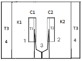 | Figure 1. Schematic representation of a calorimetric assembly including the specimen cell of heat capacity C1 and heat conductance K1 and the reference cell of heat capacity C2 and heat conductance K2. Shown are the specimen and reference crucibles 1 and 2 sitting on the tips of differential thermocouple 3 acting as temperature sensor and crucibles’ support. |
The assembly includes sample holders 1 and 2 made of 0,1 mm thick nickel or aluminium foil placed on the tips of differential thermocouple 3. The crucibles have the form of rectangular envelopes with dimensions 1x5x8 mm. They have pockets for the thermocouple tips. Thermocouple 3 carrying crucibles 1 and 2 is located in a 13x15x24 mm rectangular cavity of heating block 4.It can be seen from fig.1 that the cells have well defined surfaces of heat exchange – the flat heater wall and the flat crucible surface. These are separated by a gaseous (air) gap – the cell thermal barrier, across which the heat flows into the sample. As the geometry of the barrier and the heat conductivity of the gas as a function of temperature are known, the heat transfer coefficient K of the cell can be calculated theoretically[4]. Proceeding from the cell characteristic features, we adopt the following basic assumptions of the theory: i) the heat capacity of the gas in the gap is negligible compared to that of the crucible with sample (system), which means that the heat capacity of the cell is localized at the system; ii) the internal heat resistance R=K-1 of the system is negligible compared to that of the gaseous thermal barrier, which means that the heat resistance R of the cell is effectively located at the cell thermal barrier. In this manner, the constants K and C in equations 1-3 acquire a definite physical meaning, being spatially localized and separated. Another important consequence of the cell geometry is that due to the great difference of heat resistances of the system and the thermal barrier (1000 times and more), heat propagation across the barrier is very slow compared to that across the system. Thus, the temperature differences in the system have time to level out or become very small, making the system nearly isothermal over its surface and volume. As a consequence, the differential temperature ∆Tp in equations 1-3 is the same for any part of the system and can be measured at any point of the crucible. Another consequence is the direct proportionality of the instrument constant K to the surface Sh of the crucible, see eq.6. The sample in the crucible may fill the crucible only partially, and this will not alter the constant K, making K independent of the sample mass. An important note: a reacting sample will impart its temperature to the crucible walls (uniformly), making K independent of the reaction kinetics or thermal properties of the sample. The known geometry of the cell thermal barrier and its thermo physical parameters allows its heat transfer coefficient K to be expressed as an explicit function of the temperature 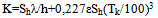 | (6) |
where the first term is the contribution to K of the heat conductivity of the gas in the gap, and the second – that of radiation (in the absence of convection); Sh is the surface of the crucible, h is the width of the gas gap, λ – heat conductivity of the gas, ε – degree of blackness of the crucible surface, conditioning its emissivity, Tk – thermodynamic temperature of the experiment. Thus, in principle, the proposed calorimeter does not need calibration, it is not dependent on other methods and in this sense is “absolute”. If, nevertheless, heat calibration is used, its purpose is to obtain more accurate results for K without recourse to eq. 6. It was shown in[4] that the theoretical K and the one obtained by calibration using pure metals are very close to each other.For a given transition according to(3,5) | (7) |
It follows from(7) that K is the measure of the calorimetric sensitivity of the instrument: the less is K, the greater is the DTA peak area At. The sensitivity increases on passing to smaller crucibles with smaller surfaces Sh. It also increases with greater gas gaps h and drastically decreases with the temperature Tk, see eq.6. The colour of the crucible is also important - black crucibles with ε close to 1 make K greater and the sensitivity lower.
2. Results and discussion
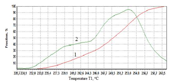
To check the conformity of the theory to practice, metrological attestation of the instrument Thermo-500 was carried out using metals In, Sn, Pb, Zn of purity 99,99XX-99,98XX mol.% and some recommendations given in[5-7]. Temperatures and heats of fusion of the metals were determined and compared with the literature values, see Table 1. Random and systematic errors of measurement were calculated, as well as their dependence on the heating rate and sample mass. For collecting experimental data a two-channel digital thermometer AZ8852 with temperature resolution 0,1oC was used. Below will be described the measurement of i) transition temperatures; ii) purity; iii) heats of transitions; iiii) heat capacities on the proposed calorimeter. This will help to highlight the major distinctive features of the proposed calorimeter as compared to the conventional calorimeters of the heat flux and Boersma DTA families[10].  | Figure 2. Heating curve of indium with operator drawn base line Tb (above) and DTA peak (below). Indicated are the initial melting temperature T1 and peak apex temperature Tm (end of melting). |
For calculating enthalpies of reactions we measure the difference ∆Tp=T1-Tb, where Tb is the base line drawn by the operator after completion of the experiment. This is the line connecting the first and last points of deviation of the experimental curve T1(t) from the linear portions of the heating curve before and after the thermal reaction in the sample, fig.2. The temperature difference ∆T=T1-T2 is measured for the special case of calculating specific heat capacities, see the corresponding section of the paper. It is highly important to have an ideally linear portion of the heating curve, coinciding with the straight base line, in the range of DTA peak, as any deviation from linearity results in greatly lowering the precision of the method.When measuring enthalpies and kinetics the thermocouples T1 and T2 can be used independently, e.g. for studying in one run two different samples, including those with close properties to establish fine differences between them in strictly similar conditions of experiment.Heats of melting are calculated using eq.3. The constant K in this equation increases with temperature, so the instrument needs to be calibrated in the working temperature range (20-500oC). For calibrating the instrument, metals with known ∆Ho and eq.3 are used, and values of K at temperatures 157, 232, 328, 420oC are calculated. After which a function K(T) of polynomial form is built using the method of least squares. For the cell described above the function turned out to be | (8) |
The program “Thermo” finds the temperature Tm corresponding to the DTA peak apex by differentiating the peak and then inserts Tm into formula 8.Accuracy and precision of the present method depend mainly on two factors – accuracy of the thermometer and the quality of the system, under which is meant its degree of isothermalness. The latter is the higher, the less is its internal thermal resistance R. It can be minimized by closely packing the sample in the crucible to exclude air pockets and bad physical contacts and by reducing the sample volume (thickness). In our case the sample is typically a 1x5x8 mm pellet. It can be packed very tightly in the crucible by pressing hard the flat crucible after filling, simultaneously a good contact of the thermocouple tip with the crucible wall is ensured. There is always a temperature lag ∆Tlag when measuring the sample temperature under dynamic conditions of the DTA experiment. It is the difference between the temperature of the thermocouple hot junction adjoining the crucible wall and the temperature of the reactant (melt) – the one we strive to determine with the greatest possible accuracy. The lag increases both with the internal thermal resistance of the system and the rate of heating, thus contributing to the systematic error of measurement. Due to ∆Tlag the measured temperature is greater than the true one during heating and less than the true one during cooling.To assess the system quality and a possible ∆Tlag one may use the melting step on the sample heating curve, Fig.3. | Figure 3. Melting step on the heating curve of indium, heating rate 10oC/min. |
It can be seen from fig.3 that the sample begins to melt at 156,0oC, and at 157oC the melting is completed. As the true melting temperature cannon exceed 156,6oC (the literature value, Table 1), we conclude that the value 157,0oC at the end of melting is due to the temperature lag ∆Tlag. It is not that great considering a rather high heating rate of 10oC/min. The quality of the system may be deemed satisfactory.The sample purity expressed in mol.% is calculated via Van’t Hoff equation | (9) |
N1=100-N2where T is the temperature along the horizontal melting step, To is the extrapolated melting temperature of an absolutely pure sample, N2 is the impurity content in mol.%, Acr is the cryoscopic constant, α is the melt fraction, and N1 is the sample purity, mol.%.Eq.9 is linear with respect to the argument 1/α. It can be approximated by a linear regression equation | (10) |
where Y=T, a=To, b=-N2/A, X=1/α. The cryoscopic constant Acr can be calculated via formulaАcr=∆Нм/R(Кm)2=∆НоМw/8,36(273+Тm)2where ∆Hm is the molar heat of melting, Km is the melting temperature in Kelvin, Mw – the sample molar mass, R is the gas constant.The melt fraction α is calculated via formula  | (11) |
where A is the current area of DTA peak, ∆Tp is the peak height (differential temperature caused by reaction), At is the total peak area, τ – cell time constant, τ=C/K found as τ=An/∆Tn, where An is the peak area taken on the exponential (tail) branch of the DTA curve, ∆Tn is its height. Eq.11 can be obtained by jointly solving equations 2, 3, and 4.Table 1. Thermodynamic Constants of Standard Samples for Heat Calibration of Thermo-500
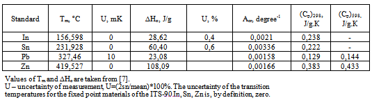 |
| |
|
Table 2. Data of Metrological Attestation of Calorimeter Thermo-500
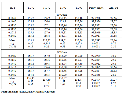 |
| |
|
In Table 2 are given sample masses, temperatures T1 and Tm corresponding to the beginning and end of melting (found from the sample heating curve T1), temperatures Ti and To, where Ti corresponds to the beginning of melting and To is the extrapolated melting temperature of pure sample, both found from eq.10. Also are given sample purity P calculated via equations 9-11 and heats of fusion ∆Ho calculated using equations 3 and 5. For all the measured quantities are given their arithmetic means, standard deviations Sn-1, and coefficients of variation CV=(Sn-1/mean)100%. It follows from Table 2 that the standard error SE=Sn-1 of all the temperatures for n=6 does not exceed 0,4oC (excepting Ti) and is the lowest for To at the heating rate of 10oC/min. SE is markedly higher for the heating rate of 20oC/min. Comparing T1 and Ti one sees that T1 exceeds Ti by about 1oC (155,5 and 154,31oC, respectively). As to Tm and To, Tm is always slightly greater than To (156,87 against 156,36oC), and both values are close to the literature value for indium Tm=156,6oC.On passing to the heating rate of 20oC/min the temperatures T1, Tm, Ti, and To remain practically the same, though their SE become bigger. The purity becomes less than 99,99XX% and its SE increases from 0,0011 to 0,0047 mol.%. Heats of fusion show little dependence on the heating rate, their CV being on the order of 3-4%.No dependence of the measured quantities on the sample mass in the interval 0,1440-0,3130 g can be detected from the data of table 2.In Table 3 are given the arithmetic means of temperatures Tm, To, sample purity P, and heat of melting ∆Ho for the number of measurements n=6. Given also are the standard deviations of measurement sn-1 and coefficient of variation CV. In the last two columns are given absolute deviations of the measured To and ∆Ho values from the literature (true) ones. Temperatures Ti and To are calculated using regression eq.10 and can be found from the graph (straight line) of the equation or the table of data left to the graph, fig.4.Table 3. Data of Metrological Attestation of Calorimeter Thermo-500
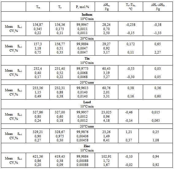 |
| |
|
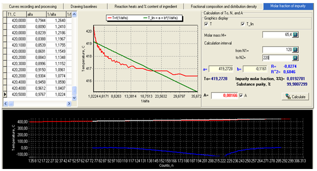 | Figure 4. Working window of module “Molar fraction of impurity” with calculation results for zinc. |
For the example presented in fig.4 we have: To=419,27 and Ti=415,13oC (1/α=35,67), regression coefficient R=0,8274. Calculated purity of zinc is P=99,9807 mol.%.It follows from table 3 that the regularities found for indium also apply to the other studied metals. The standard error of measurement sn-1 increases with the heating rate, the values of Tm and To increase by about 1oC on passing from the heating rate of 10 to 20oC/min, while purity values drop by about 0,01 mol.%. As a result the negative deviations of To from the true values at 10oC/min become positive at 20oC/min. The systematic measurement error in our case is due mainly to the instrument (thermometer) error and the temperature lag ∆Tlag (increasing with the heating rate). The thermometer gives evidently slightly lowered values of melting temperatures, as can be seen from the data for the heating rate of 10oC/min. At 20oC/min the positive systematic error due to ∆Tlag begins to overweigh the systematic thermometer error. Let us now consider the theory and procedure of the heat capacity measurements on the proposed calorimeter. Heat flow in the cell with localized C, K parameters can be described by the equations derived from the law of Newton for heat exchange. For the sample we have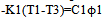 | (12) |
and for the reference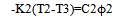 | (13) |
where K1 and K2 are the cells heat transfer coefficients, Т1 – sample temperature, T2 – reference temperature, Т3 – temperature of the heater wall, C1 and С2 – heat capacities of the systems “sample+crucible” and “reference+crucible”, 1=dT1/dt and 2=dT2/dt – heating rates of the corresponding systems. Solving equations 12 and 13 jointly assuming 1=2= and К1=К2=К, we obtain 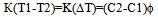 | (14) |
Where ΔТ=Т1-Т2 is the experimental differential temperature.If the sample and reference crucibles have identical form, size, colour, and mass, the coefficients K1 and K2 are the same for the two systems, hence K1=K2=K. Besides, heat capacities of the crucibles are equal. Therefore, the term C2-C1 in eq.14 is the difference of heat capacities of the reference and the sample, the heat capacities of the crucibles having cancelled out on subtracting C1 from C2. Introducing the masses of specimen and reference and their specific heats into(14) and solving for C1, we have 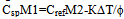 | (15) |
The specimen specific heat can be calculated fromequation 15 if Cref as a function of temperature is knownand the term ∆T/φ is found from the experiment. To calculate the change of the specimen enthalpyin the given temperature interval we integrate eq.15,obtaining  | (16) |
The term ∫KΔTdt represents the positive or negative excess enthalpy of the specimen over that of the reference, depending on the sign of ∆T. If a transition with the heat ∆Ho occurs during the run, eq.16 acquires the form  | (17) |
where ∆Ht is the total enthalpy change of the specimen, ∆Tp is the additional differential temperature caused by the transition, τ=C/K is the time constant of the specimen cell, ∆Tb is the steady state differential temperature. After integration from the start of transition to its end, viz. from ∆Tp1=0 to ΔTp2=0, the term τd∆Tp in eq.17 vanishes and thus can be omitted from final calculations (assuming τ=const during the transition).The full enthalpy change of the specimen – the left side of eq.17 is calculated by the program “Thermo” using Cref known from the literature and the experimental quantity T1-T2= ΔTb+∆Тр. The entropy change ∆Ssp is calculated via formula ΔSsp=(M2/M1)∫СrefdT2/(Т2+273)- (1/M1)∫КΔТdt/(Т1+273),and the Gibb’s free energy is given by ΔGsp=ΔHt -(T1+273)ΔSsp The procedure for conducting the heat capacity measurements is the following.Two identical crucibles are made from a 0,1 mm thick aluminium or nickel foil. A flat piece of silver weighing 0,250-0,500 g is inserted tightly in one of the crucibles and the sample is packed in the other. The sample crucible is positioned on the T1 thermocouple and the reference crucible on the T2 thermocouple. The heating program is started and temperatures T1 and T2 recorded. The program “Thermo” collects the data and calculates the sample thermodynamic parameters using formulas given above. An example of the program’s performance for zinc is presented in fig.5. In this case the sample mass was 0,23515 g and that of the reference (silver) 0,3450 g, the heating rate 15oC/min, atmosphere in the oven– air.As can be seen from fig.5, the program presents calculation results in graphical and tabular form. Besides, the overall change of thermodynamic functions: enthalpy, entropy, and Gibb’s free energy in the temperature interval studied is given in the space above the table.The data in fig.5 for the specific heat of zinc show a close agreement with the literature data, see Table 1. In general, the average absolute error of measurement by this method may amount to 0,02-0,03 J/g.K.Under the curve of zinc is drawn the heat capacity curve of silver calculated from the literature data.In fig.6 are given data on the heat capacity of polyethylene terephthalate (PET) – a polymer often used for demonstrating the working capabilities of various DSC instruments. Figure 6 shows a two-step glass transition at 70-80 and 80-105oC, a two-step crystallization at 118-130oC and 130-135oC, and a two-step melting at 217-245 and 245-260oC.For better viewing the region of the glass transition of PET a narrow temperature interval 43-115,6oC was selected for calculations, fig.7.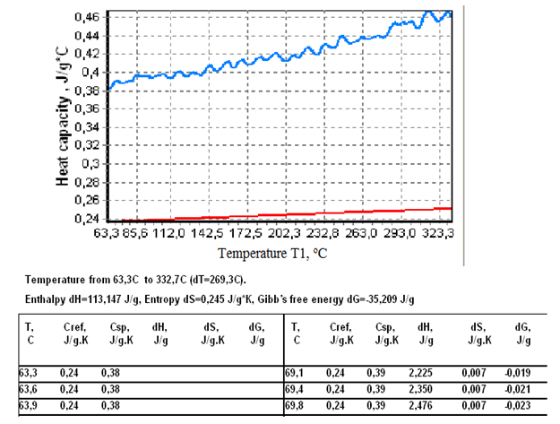 | Figure 5. Heat capacity curve of zinc in the interval 63,3-332,7oC. |
 | Figure 6. Heat capacity of PET in the interval 49,7-288,1oC. |
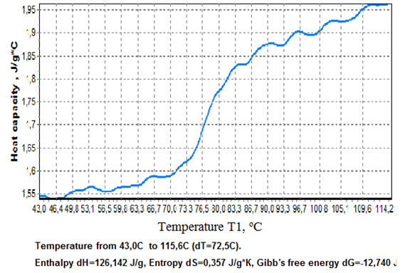 | Figure 7. Glass transition of PET viewed in greater detail than in Fig.6. |
Figure 7 shows an increase of Cp of PET at 70-87oC by 0,25 J/g.K flanked by a small Cp increment at 50-70oC (0,05 J/g.K) and a larger one at 85-110oC (0,10 J/g.K). In order to calculate the heats of crystallization and melting of PET, experimental data was presented in the format of conventional DTA curves, fig.8. 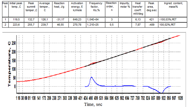 | Figure 8. Data for PET presented as conventional DTA curves ∆Tp(t). |
 | Figure 9. Crystallization peak of PET viewed in greater detail than in figure 8. |
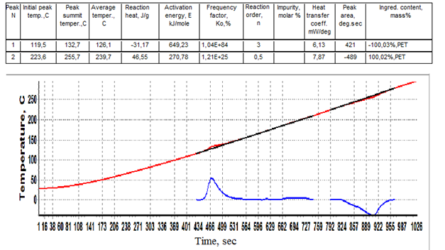
 | Figure 10. Integral (1) and differential (2) thermal stability distribution curves of PET crystals derived from melting DTA peak. |
The baseline for the crystallization peak was drawn from 119,5 to 210oC and for the melting peak from 223,6 to 260oC. The summit peak temperatures of crystallization and melting 132,7 and 255,7oC and heats of crystallization and melting -31,2 and 46,6 J/g were found, see the table of calculation results above the curves of fig.8. In fig.9 the crystallization peak is presented in greater detail as a function ∆Tp(Tb). A second small crystallization peak at 180-210oC can be observed on the differential curve indicative of further ongoing crystallization processes in PET at temperatures just preceding melting.It would be of interest to assess the distribution of lamellar crystals in PET according to their size (thermal stability) assuming that small unstable crystals melt first and the more stable large ones melt last. For this it is sufficient to plot the melt fraction α against the temperature T1 or Tb and then differentiate the integral curve, fig.10.It can be seen from fig.10 that about 45% of PET crystals form a low size fraction melting at 230-245oC, and the remaining larger size fraction melting at 245-260oC. The distribution is tri-modal, with modes centered at 240, 249, and 253oC. The relative amounts of each fraction can be found from the integral distribution curve.For studying the kinetics of crystallization and melting of PET on the proposed absolute calorimeter the following procedure is used. First, the kinetic law of phase transformation is postulated in the form of a power function of α | (18) |
then, transforming equation (18), we haveB=(d/dt)/(1-)n =Ko*exp(-E/RT)  | (19) |
Degree of conversion α is calculated via formula (11). Equation (18) is an equation of linear regression | (20) |
The constants a and b are calculated by the program “Thermo” using the method of least squares. The exponent n (reaction order) is varied by the operator until a value of the regression coefficient Rr closest to 1 is obtained. The kinetic constants corresponding to the best n value are accepted as the true ones.The results of such calculations for PET are summed up in the table of fig.8. The exceptionally large values of Ko=1,04 1084kJ/mol and E=649 kJ/mol (n=3, Rr=0,9912) point to a very rapid crystallization process of explosion-like type (cooperative self-assisted crystallization). The melting of PET proceeds in a more quiet manner with Ko=1,21 1025 and E=270,8 kJ/mol (n=0,5, Rr=0,9750).
3. Conclusions
An absolute heat conduction calorimeter of isolated container type has been developed. Its characteristic features are:A simple and robust design of the calorimetric assembly making possible heating to 1000oC or higher without damage of the assembly.Effective thermal (physical) isolation of the sample container from the heater and support has resulted in a highly isothermal calorimetric system making possible mathematical modeling of the cell and derivation of all the calculation formulas from the model.Direct precise reading of the sample temperature is possible without recourse to multiple heating rates calibration due to the tight intimate contact of the sensor with the nearly isothermal calorimetric system (sample holder with sample).The instrument (calibration) constant K can be obtained either theoretically from the known thermo physical parameters of the cell or by enthalpy calibration. It depends on the size and colour (emissivity) of the sample container, temperature, and does not depend on the sample mass or its nature (metal, organic, inorganic) or the heating rate. A single time constant of the instrument is sufficient to characterize its thermal inertia (response time). It typically lies between 5-10 sec for high temperatures and 20-30 sec for low ones.The calorimetric sensitivity of the instrument is directly given by its calibration constant K and is rather high due to the low heat conductance of the cell gaseous thermal barrier. Therefore, no electronic amplification of the recorded signal is needed. Heat capacities, reaction heats, kinetic constants, purities are obtained simultaneously and in one run – no multiple runs or multiple calibrations are needed. No desmearing of recorded DTA curves is needed thanks to the high resolution of thermal events in the system with low temperature gradients and true sample temperatures recorded. Metrological attestation of the instrument has shown its ability to measure: temperatures with the relative uncertainty u=0,2-0,4%, where u=(2sn/mean)100%, ii) purity withCV=0,0011-0,0070%; iii) fusion heats with CV=3-5%; iiii) heat capacities with an average absolute error 0,02-0,03 J/g.K.
References
| [1] | Shishkin Yu. L., Isothermal-surface transmitter with thermally insulated sample holder. A novel approach to quantitative differential thermal analysis.,1984, J. Thermal Anal. Vol. 29. N1.P. 105 – 113 |
| [2] | Shishkin Yu. L. The instrument constant in DTA. Theory of sensing units in DTA instruments ., 1986, J. Thermal Anal. Vol.31, N4. P. 917 – 930 |
| [3] | Shishkin Yu. L. The instrument constant in DTA. Theory of sensing units in DTA instruments. An introduction to time-space calorimetry., 1987, J. Thermal Anal. Vol. 32. N1. P.17 – 34 |
| [4] | Hohne G., Hemminger W., Flammersheim H.-J., Differential Scanning Calorimetry, Springer-Verlag,Berlin/Heidelberg/New York, 2003 |
| [5] | Gmelin E. and Sarge St.M., Calibration of differential scanning calorimetrs., 1995, Pure & Appl. Chem. V.67, P. 1789-1800 |
| [6] | Giuseppe Della Gatta, Michael J. Richardson, Stefan M. Sarge, and Svein Stolen., Standards, calibration, and guidelines in microcalorimetry. Part 2. Calibration standards for differential scanning calorimetry (IUPAC Technical Report)., 2006, Pure & Appl.Chem. Vol. 78. N7. P. 1455 – 1476 |
 Abstract
 Reference
 Full-Text PDF
 Full-Text HTML