1. Introduction

Before the invention of cars, journeys took hours, days and even months but now a weeks' journey can be made with a return on the same day. Since the invention of the first gasoline powered automobile in 1886 [1], the lifestyle of humans has evolved around the use of cars to transport us and our properties. The world has continuously been adapting to the use of cars by constructing facilities such as roads, bridges and interchanges that makes the use of cars more efficient and save travel time. This new efficient way of travelling comes at a cost to the traveler. A service fee also known as transport fare is paid by the passenger to the operator of the vehicle. Oxford University Press defines fare as “the money that you pay to travel by bus, plane, and taxi” [2].

To the traveler, transport fare is the amount paid for the distance a public transport service is aiding to cover which makes the cost directly proportional to the distance covered. This costing type is called linehaul cost and is defined by [3] as costs that are a function of the distance over which a unit of freight or passenger is carried. Transport fare impact on many activities of the country especially commodities that are transported by vehicles with high transport cost contributing to the continuous rise in the price of consumable commodities [4].

Several research have been conducted in relation to transport in the Ashanti region but not much attention has been paid to analysing transport cost. This paper seeks to analyse using time series the transport fare over the years in Kumasi.

To the service provider, transport fare is more than just the distance covered and entails the cost of operating and maintaining the machine. Several factors such as fuel cost, repair and maintenance cost, labour, spare parts, road conditions and the distance covered, and regulations affects the pricing of a journey [3]. A study by [4] links transport cost to bad roads, illegal collection of money by highway patrol team, high price of motor spare parts and high fuel prices.

In Ghana, road conditions are perceived to increase transport cost, by the increase in fuel consumption, maintenance costs and reduce the life of trucks [5]. Studies into the West African corridor discovered that, if international corridor routes are paved and in reasonable condition, further improvement of road conditions do not result in significant reduction of transport costs [5].

[6] observed that an increase in spare parts cost increases transport fare. His study finds that the high import duties prevailing in the county impacts adversely on the sales and quantity of spare parts imported into the country. This means that the price of spare parts in the country will be high and translate into high transport fares in the country [6]. Most countries import their spare parts which makes the pricing affected by the currency exchange rate and the importation tax on the parts. And with the Ghanaian economy having a persistent depreciation of the cedi [7], [8] suggests that the exchange rate depreciation is a potentially important source of price inflation in Ghana with the pass-through to consumer prices substantially high.

Public transport fare in Ghana is regulated by the Ghana Private Road Transport Union (GPRTU) in deciding the rate for taxis and minivans but ride-hailing platforms such as Uber, Bolt and In-Driver have their own pricing model. Studies such as [9] on spatial disparities of urban public transport fares in Kumasi revealed that an extreme price variability and inconsistent pricing of transport indicating that two passengers traveling the same distance on different route can pay drastically different prices. Ride hailing has introduced a new method of transport pricing for passengers and drivers. The advent of ride-hailing has revolutionized transport pricing. Scholars have analyzed this shift from various angles: [10] examined platform profitability and pricing structures in the Chinese market, while [11] investigated optimal dynamic pricing strategies.

Petrol and diesel are the main fuel used by commercial drivers in the Ghana and fluctuations in the fuel price affects the fare of the passengers and as such can have effect on the behavior of the people in making a journey [12]. Although fuel price is directly link to transport fares, a research by [13] on fuel consumption and distance charges shows that passengers are undercharged on some routes whereas they are overcharged on others. Oil price and transportation is a topic that has received much attention and numerous articles can be found on the topic. The study by [14] examines the relationship between oil price fluctuations and transport costs, culminating in a model for predicting future oil prices. According to [15] a small but consistently significant amount of transit ridership fluctuation is due to gasoline prices.

With the increasing rate in cost of transport fare, some analyst and researchers have proposed free transport policies or transport incentives to reduce the burden on the people. A research caried out by [16 ]on bus fare exemption for the young discovered that bus travel can be both a physically and socially active experience for young people. The research by [17] demonstrates an inverse relationship between bus fare and demand, showing that lower fares result in higher ridership.

There has been a lot of research related topics on transport and transport fares but not much has been done about the time varying factor of transport fare. Through a time-series analysis of ridership, [15] provides a framework to guide pricing policy. Similarly, [18] emphasized that “time series analysis can provide valuable insights into the fluctuations of ridership and the factors influencing demand”. [19] further advanced this approach by applying big data analytics to model bus passenger demand, demonstrating the adaptability of time-series methods in contemporary transport research.

Rising transport costs exert a significant burden on passengers’ expenditures, particularly in contexts where income levels remain stagnant or wage adjustments fail to align with fuel price increases. Before the 2021 adjustment, the Labour Department increased compensation of employees by 13.68% in the 2019 budget [20]. The most recent adjustment to public sector salaries occurred in July 2021, when the government implemented a 4% increase in the base pay following negotiations with the Public Service Joint Standing Negotiating Committee [21].

This increase in income does not match the increase in transport fares in the country. On January 17^th, 2022, transport fare witnessed an increment of 40% [22] which is far from the increase in income. Fuel prices have been rising over the years and is directly affecting the transport economy and transport fare. The recent hike in fuel price and transport fare has been attributed to the Russian-Ukraine war by the media and many analysts [23]. [24] discovered that the invasion of Ukraine has increased the prices in important commodity market.

Since 2014, the United States, the EU, and other international actors have applied economic sanctions on Russia in response to its policies toward Ukraine [25]. The sanctions of the western world on Russia have contributed to the hikes in fuel due to Russia being a major oil and natural gas for Europe [26]. The lack of oil coming from Russia means a drop in the supply on the European market with the demand not increasing. This phenomenon is affecting the globe entirely as Russia remained a global of oil and gas until the sanctions hence the rapid increase in transport fare. According to [27] report on oil market and Russian supply, Russia is the world’s largest exporter of oil to global markets and the second largest crude oil exporter.

The public transport market in Ghana is made up of vehicles such as minivan for both intracity and intercity travel, taxis for intracity travels and buses for intercity travels. Although intracity buses reduces congestion and cost 20% less than the minivans, the public prefers to travel by the minibus instead of the more cheaper Metro Mass Transit [28]. [28] recommend strategies for Metro Mass Transit to increase ridership, noting that, with fares set lower than alternative modes of transport, ticket prices can remain affordable for passengers while improving service uptake.

The government of Ghana in 2016 introduced a bus system called the Ayalolo by the public to curb traffic and serve as reduce cost in travelling [29]. Traveling by bus is an efficient mode than minibuses and taxis [28].

[30] provides an analysis of the choice of transport method by the passengers of Kumasi. In their research they recommended the use of large occupancy vehicles such as buses. The data from their research shows taxi as the dominant preferred means of travel by passengers bosting more than 44% of the market even though it has higher transport fare relative to the other means.

The introduction of auto-rickshaws in Ghana has provided a new mode of transport for passengers. While these operators often exhibit low compliance with road safety and traffic regulations [31] demand for auto-rickshaws continues to grow across African urban transport markets [32].

Various policies and operations have taken place over the years to reduce the operation cost of transport operators thereby reducing transport cost. In 2014, World Bank approves $25 million in new financing from the International Development Association (IDA) to support the Government of Ghana’s effort to improve the mobility of goods and passengers on selected roads through reduction in travel time, in vehicle operating costs and enhanced road safety awareness. The finance was geared toward improving the poor infrastructure which impedes the mobility of goods and passengers and create high transport costs [33]. [5] in their publication on transport prices and cost in Ghana recommended that the most effective measures to reduce transport costs are likely to be a decrease of fuel costs and an improvement of road condition.

Transport fares in Ghana, unfortunately, is not governed by strict regulation or policy, and this makes fares unpredictable. To this end, this study seeks to model transport fares in Ghana, through distance-based approach, using evidence from Kumasi metropolis.

2. Materials and Methods

2.1. Study Area

The Ashanti Region is located in the central part of Ghana and comprises 43 local government assemblies, including one metropolis, 18 municipalities, and 24 districts (MMDAs). Geographically, it lies between longitudes 0° 9′ 0″ W and 2° 15′ 0″ W, and latitudes 5° 30′ 0″ N and 7° 27′ 36″ N. According to the 2021 Population and Housing Census, the region has a population of 5,432,485, covering approximately 10.2% of Ghana’s total land area of 24,389 square kilometres. Its central location enhances its strategic importance for national and international supply chains. The road network connects Kumasi to major cities such as Tamale via Techiman and Yeji, with Techiman also linking to Wa in the Upper West Region. Additional roads provide access from Kumasi to Sunyani, Koforidua, Accra, Cape Coast, and Takoradi [34].

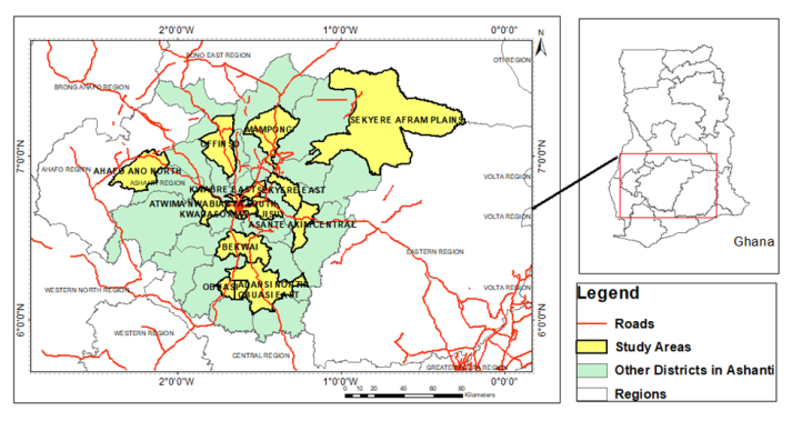Figure 1. Mapping Representation of Study Area

2.2. Source of Data

Quarterly secondary data on transport fares was obtained from the Ghana Private Road Transport Union (GPRTU) covering the period from January 2015 to December 2024. Quarterly data were used because Ghana’s petroleum deregulation policy, which influences fuel prices and consequently transport fares, is implemented on a quarterly basis. The dependent variable, Transport Fare, was measured in Ghana cedis (GHS) as the officially approved average fare charged to passengers for travel by commercial minivans over designated urban routes within Kumasi. The fares were recorded as nominal values; no adjustments were made for inflation in the present analysis.

The independent variables were the median distance of 5.3 km, representing the median length of selected representative urban routes within Kumasi measured in kilometres, and the mean distance of 5.7 km, representing the average length of the same set of routes. No transformation was applied to these variables before modelling, as the analysis employed differencing within the ARIMA framework to achieve stationarity.

2.3. Regression with ARIMA Errors

The regression with ARIMA errors was adopted for modelling the data because the response variable exhibits a linear relationship with the covariates while the exogeneous variable shows time series structure. Through this model, the ARIMA model with the error parameter, it captures both the direct impact of the predictors and the autocorrelation patterns relative to the residuals.

Therefore, suppose that is the response variable which has a linear function of predictors and and as well as an ARIMA (5,1,0) error term. This is given as follows:

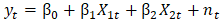(1)

where:

= transport fare (GHS) at time t

= median route distance (km) at time t

= mean route distance (km) at time t

= error term following an ARIMA (p,d,q) process

The ARIMA (p,d,q) error term is defined as:

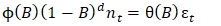(2)

where:

= autoregressive polynomial of order 5

= backshift operator

= white noise error term

2.3.1. Model Fitness Test

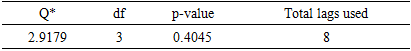
Among others, the Portmanteau (Ljung-Box) test was utilized to test the following hypothesis:

: The residuals are distributed independently

: The residuals exhibit serial correlation

Using the test statistic;

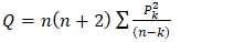(3)

Where is the sample size, is the sample autocorrelation at lag , and follows a Chi-square distribution with degrees of freedom,

3. Results

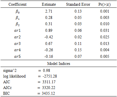
It is noteworthy that transport fares in Ghana, and especially withing Kumasi metropolis, is distance-based. Following the analysis of the data using the auto.arima() function in R version 4.3.3 to straight away identify the best-fit regression with ARIMA errors model, the ARIMA (5,1,0) errors was obtained as follows:

Table 1. Coefficients of Regression with ARIMA (5,1,0) errors

The regression with ARIMA (5,1,0) model was derived from Table 1 as follows:

(4)

and

(5)

Stationarity was achieved after the first difference as shown in Equation (5). The regressors, median distance (5.3km) and the mean distance (5.7km), were significantly contributing to transport fares Kumasi metro. This assertion was supported by the standard errors of the estimates 0.05 and 0.03 for 5.7km and 5.3knm respectively. Moreso, for every change from one quarter to another, transport fares increased by 0.28 (28%) and 0.31(31%) for the 5.3km and 5.7km distances respectively.

Also, the AR estimates; were each significant at with minimal standard errors 0.06, 0.02, 0.11, 0.0.15 and 0.07 respectively.

The AIC figure of 3311.17 indicates that the regression with ARIMA (5, 1, 0) error dynamic model was the notable pick among all possible array of similar models since it produced the smallest AIC figure as opposed to the rest. The AICc and BIC figures of 3320.22 and 3435.12 respectively corroborate the informed choice of the model as they were the least figures with that domain.

Table 2. Portmanteau Test for Residuals from Regression with ARIMA (1,0,3) errors

The p-value (0.4045), as shown in table 2, is greater than the margin of error (5%). This provides no basis for the rejection of the null hypothesis. Thus, the residuals were independently distributed at 95% confidence interval. This means that the residuals do not serial autocorrelation, which is an indication that prediction domain yielded accurate coverage within the 95% confidence interval. It is worth noting that all the error parameters; RMSE, MAE, MAPE, and MASE yielded values far less than 1, which further confirms that the coefficients obtained were appropriately estimated.

The ACF, as shown in Figure 2, demonstrates that the series achieved stationarity after the first difference within the estimated boundary while the histogram exhibits, largely, an appropriate interval for purposes of prediction.

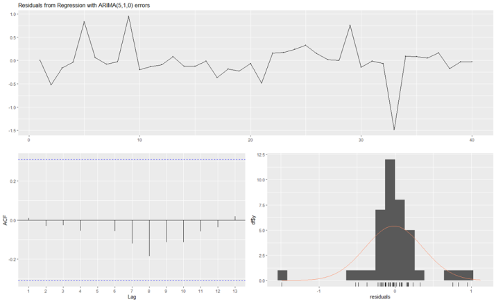Figure 2. Regression with ARIMA (5,1,0) residual diagnostics

From Figure 3, the forecast for Q1-2025, Q2-2025, Q3-2025, Q4-2025, Q1-2026, Q2-2026, Q3-2026, and Q4-2026 were 10.10, 12.30, 14.15, 15.90, 17.10, 17.80, 18.30, and 19.25 Ghana cedis respectively.

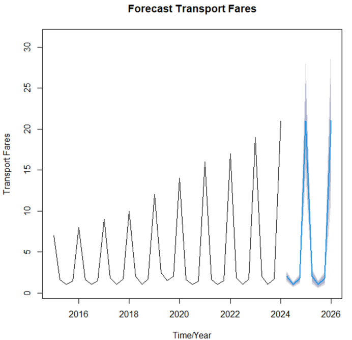Figure 3. Forecast for regression with ARIMA (5,1,0)

4. Discussion

The results of this study indicate that the regression with ARIMA (5,1,0) errors provides a robust framework for modelling transport fares in the Kumasi Metropolis. The significant contribution of median and mean distances (5.3 km and 5.7 km) to fare determination aligns with [15 who found that fare structures in Ghana are often distance-sensitive but can vary considerably between routes. Similarly, a study by [15] confirms that transportation pricing dynamics are not solely a function of fuel price trends but are also shaped by other operational and structural factors.

Compared with earlier work by [5], the current findings reinforce the argument that improvements in road quality, while important, may not always translate into substantial fare reductions unless accompanied by broader interventions, such as regulating fuel costs or rationalizing spare parts pricing. The presence of quarterly spikes in the forecasted fare pattern mirrors findings by [4], who observed volatility in transport costs as a result of fuel price deregulation and seasonal demand fluctuations.

An unexpected observation was the persistence of fare increases even in periods where distance remained constant. This suggests that non-distance determinants, such as currency depreciation, inflationary pressures, and informal levies, may exert considerable influence on fare pricing. These factors have been highlighted by [8] and [7] as important drivers of price instability in Ghana.

The forecast results, which indicate a gradual upward trend with intermittent spikes up to the last quarter of 2026, have important policy implications. Stakeholders, particularly the Ministry of Transport, the Ghana Private Road Transport Union (GPRTU), and municipal authorities, could use these projections to plan interventions such as fare stabilization funds, targeted fuel subsidies for public transport operators, or the introduction of flexible fare caps to protect vulnerable commuters. Furthermore, the adoption of more fuel-efficient and higher-occupancy transport modes, as suggested by [30] could moderate future fare hikes.

Despite the promising results, this study has certain limitations. First, it relies solely on secondary data from the Motor Traffic and Transport Department (MTTD), which may not capture informal fare adjustments or regional variations in pricing. Second, the analysis did not adjust for inflation, meaning that the real purchasing power implications of fare changes were not fully assessed. Third, the model focused primarily on distance as a determinant, potentially omitting other critical variables such as fuel price, road conditions, vehicle maintenance costs, and policy changes. Future research could address these limitations by incorporating primary data collection, applying inflation-adjusted fare indices, and expanding the range of explanatory variables to develop a more comprehensive transport fare forecasting model.

5. Conclusions

Among all possible similar models, the regression with ARIMA (5,1,0) errors was the best model in estimating transport fares from the first quarter of 2015 to the last quarter of 2024. The regressors of transport fares, 5.3 km and 5.7 km, were significant in modelling transport fares over the period concerned. The forecast figures, which extend to the last quarter of 2026, reflect an up-and-down pattern with occasional spikes.

In view of these findings, stakeholders including individual drivers, drivers’ unions, the Ministry of Transport, and research institutions should consider targeted measures to reduce the volatility of transport fares. Policies such as fare stabilization mechanisms, periodic review of operational costs, and promotion of high-occupancy public transport could help protect commuters from sharp increases in price and improve affordability within the Kumasi Metropolis.