-
Paper Information
- Paper Submission
-
Journal Information
- About This Journal
- Editorial Board
- Current Issue
- Archive
- Author Guidelines
- Contact Us
International Journal of Traffic and Transportation Engineering
p-ISSN: 2325-0062 e-ISSN: 2325-0070
2020; 9(2): 25-36
doi:10.5923/j.ijtte.20200902.01

Quantify the Relationship Between Roundabout Geometry and Delay
 Abstract
 Reference
 Full-Text PDF
 Full-text HTML
Nikolay Nazaryan, F. Clara Fang
Department of Civil, Environmental and Biomedical Engineering, College of Engineering, Technology and Architecture, University of Hartford, West Hartford, CT, USA
Correspondence to: F. Clara Fang, Department of Civil, Environmental and Biomedical Engineering, College of Engineering, Technology and Architecture, University of Hartford, West Hartford, CT, USA.
| Email: |  |
Copyright © 2020 The Author(s). Published by Scientific & Academic Publishing.
This work is licensed under the Creative Commons Attribution International License (CC BY).
http://creativecommons.org/licenses/by/4.0/

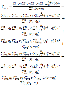
This paper reports about an investigation of the effect of the length of an additional approaching lane of a roundabout on the delay. To calculate delay, a mathematical algorithm has been developed, representing dependence of velocity  a traveling vehicle on its traveling distance
  The study shows a mathematical algorithm which can supply more accurate and simpler calculations, represented through the sixth-degree polynomial function possessing just three extrema points: a maximum and two minimums. It is shown that application of data collection on existing additional lanes, performed during different periods of time during weekdays will allow us to obtain the family of curves
  , where each curve will have its own individual extrema points with the consequent coordinates
  and
and  These curves, obtained on the base of the analytical function and the practical data collection, will allow road engineering experts to design a roundabout’s additional approaching lane and to estimate the proper delay with the very high degree of accuracy.
Keywords: Roundabout geometry, Delay, Mathematical algorithm, Velocity, Traveling distance, Sixth-degree polynomial function, Extrema points, Family of curves
Cite this paper: Nikolay Nazaryan, F. Clara Fang, Quantify the Relationship Between Roundabout Geometry and Delay, International Journal of Traffic and Transportation Engineering, Vol. 9 No. 2, 2020, pp. 25-36. doi: 10.5923/j.ijtte.20200902.01.
Article Outline
1. Introduction
- The object of this proposal is to develop a mathematical model, based of kinematics, which can represent the dependence of the delay of vehicles from the length of an additional lane, approaching and/or departing roundabout. In design of the modern roundabouts it is added the second lane to the urban street (taper), approaching to the roundabout. This circumstance allows significantly decrease the capacity of each lane and decrease by this way the delay of vehicles. The length of a double-entry (or exit) lane is the one of the main factors affecting on the delay of the vehicles. Therefore, considering the delay as the degree of usefulness, in this work have been analysed the length of the additional entry lane, which also can be used for analysing the additional exit lane. This study may have large application in transportation engineering design of the lengths of the additional entry/exit lanes of the modern roundabout’s performance. Despite of that the design of an additional lane differs from a flared entry, however the results of this study can also be applied to flare lengths if they are designed to operate in a similar fashion as additional lane entry. The modern roundabout has become an increasingly popular form of intersection control in the United States due to its effectiveness in improving safety and reducing traffic congestion. Since the first modern roundabout was built in Nevada in 1990, the number has increased significantly, and as of December 2012, more than 2,000 have been constructed [1].As roundabouts have become increasingly popular in the United States, it is very important to establish some means of improving their performance soon when vehicle demand nears or exceeds capacity. At signalized intersections, U.S. transportation professionals regularly consider parameters such as green time, cycle length, and number of lanes in order to improve traffic operation. However, there has not been much research performed domestically that addresses how to vary different geometric parameters to improve operations for a roundabout when analysis shows that a nearby development will impact traffic operation. Hence, most transportation professionals refer to studies conducted overseas that do not necessarily translate directly to domestic roundabout design and operation. One of the design requirements that needs further exploration is the entry approach. The entry can be designed to increase capacity either by adding a full lane upstream of the roundabout or by widening the approach gradually (flaring) through the entry geometry [2]. Most of the studies on roundabout entry design have been looking at the widening effect of the width of the approach lane. However, little attention has been given to the length of the approach and its effect on roundabout operation. The National Cooperative Highway Research Program (NCHRP) report on roundabout design neither provides recommended lengths nor gives information on how long the entry lane needs to be widened along the approach. The Federal Highway Administration (FHWA) roundabout guideline, which was superseded by the NCHRP report, suggests a minimum flare length of 80 feet in urban areas and 130 feet in rural areas [3]. It is not clear whether the suggested flare length also applies to additional lane design, and the maximum flare length is not specified. In general, the increasing popularity of roundabouts in the United States underscores the need for more research on roundabouts in the United States to address the issues that traffic engineers face in practice. The means of improving signalized intersections to meet specified demands have been well researched and documented, and methods for predicting their performance are well established. However, roundabouts lack such research on performance improvement. Our investigation will examine the effect of additional lane lengths on a double-lane roundabout operation using delay as the primary measure of effectiveness. The study is intended to provide transportation professionals with a means of improving existing roundabout operational performance and to aid the planning and design stages so that future roundabouts can be built with appropriate lane lengths to yield better performance. When compared to signalized intersections, then research available on improving operations at roundabouts due to increased traffic flow is comparably lacking. Signalized intersections usually implement several modifications to improve safety and performance over time due to new developments or increases in traffic flow. Since roundabouts handle traffic flow similarly to signalized intersections, it is possible for the volume-to-capacity
 ratio to approach or exceed 1.00. Under such conditions, long queues form, and delay increases at roundabouts. Such conditions require modifications to improve performance. Earlier research on roundabout operation was conducted by the United Kingdom–based Transport and Road Research Laboratory (TRRL), where numerous experiments and observations were performed on existing roundabouts. Kimber incorporated findings from the TRRL studies and identified six geometric parameters as having a significant effect on capacity: entry width, approach half-width, effective flare length, flare sharpness, inscribed circle diameter, and entry radius [4,5]. Out of the six parameters, entry width, approach width, and flare length were determined to be the most relevant with regard to capacity.The approach width, typically 12 feet in the United States, is the width of the travelled way in advance of any entry flare; the entry width is the width of the travelled way at the point of entry. FHWA identifies the entry width as the “largest determinant of a roundabout’s capacity” [3]. NCHRP recommends an entry width of 24 to 30 feet for two-lane entry and 36 to 45 feet for three-lane entry. It does not, however, specify how far back the additional lane or flaring should begin. In Europe, where flaring design is more common than an additional lane design, the U.K. Department of Transport Design Manual recommends flare lengths of about 82 feet (25 meters) for widening to effectively increase capacity [6]. Flare lengths greater than about 328 feet (100 meters) result in higher speeds, which undermines the main purpose of the modern roundabout configuration. The configuration of a modern roundabout reduces driver approach speeds to improve safety and enhance traffic flow. Therefore, when increasingly long lane lengths are used, the safety benefit of roundabouts may be forfeited. The 82-foot recommendation by the U.K. Department of Transport Design Manual has not been tested in the United States, but some state agencies follow the overseas guidelines, since data on the additional lane or flare length have not been provided. Interim requirements and guidance on roundabouts by the New York Department of Transportation suggest a flare length of 41 feet (12.5 meters) to 328 feet (100 meters) for urban areas and 66 feet (20 meters) to 325 feet (100 meters) for rural areas [7]. The FHWA used a model developed by Wu [7] in determining the capacity of a roundabout, whereby short length widening at the approach is considered [3,8]. Wu estimated the capacity of an unsignalized crossroad and T-junction intersection by taking into account the length of the turn lanes. Wu later analysed this model at a roundabout intersection and introduced an enhancement/correction factor for determining the capacity of a double-lane entry at a roundabout [9]. Wu was able to identify the effect of entry length, but the effect of the additional lane length at the exit was not mentioned, and it was assumed that the capacities of both lanes were identical and the traffic flow in both lanes at the entry was equally distributed. However, studies conducted on some double-lane roundabouts in the United States show that the right lane is utilized more frequently than the left lane and thus is usually considered to be the critical lane. For instance, one of the double-lane roundabouts in Brattleboro, Vermont, showed that the right lane had about 70 percent of the entry total flow, so capacity in the Wu model appears to have been overestimated [10]. This research examines the effect of the flare/additional lane length on roundabout operation using typical U.S. driving behaviour, where the right lane is considered the critical lane and is utilized more frequently than the left lane. In order to model typical U.S. driving behaviour, VISSIM was used for analysis purposes. VISSIM is a microsimulation software from Germany in which vehicles are modelled using parameters such as driver behaviour, vehicle speeds, and vehicle type [11]. VISSIM has the ability to control gaps and headways on a lane-by-lane basis to accurately replicate vehicle operations at roundabouts. Numerous studies have used VISSIM microsimulations to examine roundabout performance due to their unique ability to mimic real-world traffic operations. Trueblood and Dale considered VISSIM to be a very effective microsimulation software package for roundabout performance analysis and used VISSIM to model existing roundabouts in the state of Missouri [12].Bared and Afshar used VISSIM to model roundabouts for various ranges of circulating and entry traffic volumes [13]. They found that simulation results from VISSIM matched field data more closely than those from the SIDRA analytical and RODEL empirical models. The additional lane lengths that were analysed in VISSIM for both scenarios included 0 feet, 150 feet, 250 feet, 350 feet, 450 feet, and 550 feet. The VISSIM lane closure feature was utilized to make the zero-foot length possible. While reducing the exit and entry lanes on a double-lane roundabout to a single lane is not practical, and study in [14] illustrated that the extent of the delay effects up to zero feet.
2. Literature Review
- The purpose of paper [15] is to provide insight as to how additional lane length on an approach and/or departure affects roundabouts. Continuing of this investigation authors of paper [16] showed that there is a general notation among transportation professionals that having a longer additional lane length at a double-lane roundabout entry yields better performances. Here this notation has been investigated on the base of Lighthill-Whitham-Richards Model Analysis. Using Lighthill-Whitham-Richards Model, a double-lane roundabout with additional lane design at the entry is analyzed. The additional lane lengths are varied at the entry in order to study the effect of different additional lane lengths on roundabout performance. A scalar hyperbolic partial differential equation (PDE) model for traffic velocity evaluation, based on seminal Lighthill-Whitham-Richards (LWR) ODE for density is used. It is show that from the analysis presented in this paper, the delay and the speed can be predicted from knowledge of the geometric parameters. However, in our work, we have developed another mathematical model which is built-in a way when following parameters of the double-entry roundabouts are considered: the length of its ramp, the speed/kinematics of vehicles, the length of vehicles, moving on the ramp, the acceptable gap between consequent vehicles, and the time spending each type of vehicle to merging with the roundabout traffic flow. There are plenty works, domestic as well as foreign authors, related to the investigation of capacity of roundabout entry and delay. Authors in [17] showed that in addition to circulating vehicles, pedestrian flow is another key conflicting stream which has significant impact on entry capacity. The pedestrian impact is considered by an adjustment factor in the existing method which was developed based on the roundabouts under the design with physical splitter island, crosswalk and distance of one-vehicle length between crosswalk and yield lane. In work [18] authors used an empirical approach to develop a capacity reduction coefficient as a function of the volume of circulating vehicles in front of the subject entry and the volume of crossing pedestrians. Based on data collected at roundabouts in Germany, different expressions were developed for the cases of single-lane and two-lane approaches. According to these expressions, the effect of capacity reduction, caused by pedestrians, increases with pedestrian volume (for given circulating flow) and decreases with increasing circulating flow (for given pedestrian volume). It was shown that pedestrian crossings do not affect entry capacity at all for circulating volumes over 900 pcu/h and 1600 pcu/h (pcu-passenger car unit), respectively for single-lane and two-lane approaches. Based on the observed data authors in [19] evaluated the performance of capacity estimation for single-lane roundabouts using the Highway Capacity Manual (HCM) 2000 model. In this study, the HCM 2016 model is indicated to be over or under-estimate roundabout entry capacity. The reason of this because the HCM 2016 model estimates capacity using an unfit assumption of headway distribution type. Estimation of roundabouts entry capacity by considering pedestrian impact through several influencing factors, such as pedestrian approaching side, farside pedestrian recognition rate (FPRR) of drivers, and physical splitter island is done in [20]. The impacts of these influencing factors are examined by microscopic simulation in this study. Results from the simulation study showed that under the condition without a physical splitter island, entry capacity was reduced more significantly when more pedestrians were from the farside of the crosswalk, whereas capacity relatively increased with decreasing FPRR. Furthermore, entry capacity was also increased after the installation of a physical splitter island. Because in suburbs of Australia the single-lane modern roundabouts are one of the most important intersection types, so based on it the paper [21] is dedicated to estimation of their entry capacities. In this case the study, and the analytical model based on the gap acceptance theory by incorporating the effects of the exiting vehicles is proposed. Then, a scenario analysis is carried out to assess the effects of the exiting indicators. The results show that the transport authorities need to strictly enforce the use of indicators before exiting in order to achieve higher capacity. Author of paper [22] have developed a gap acceptance model for roundabouts that takes into consideration the proportion of exiting vehicles. It was assumed that exiting vehicles are influencing the gap acceptance process in the following way: when they leave the roundabout, new gaps that consist of combinations of old gaps arise. The distribution of the new gaps is obtained by a convolution of the distribution of the old gaps. It is shown that the proportion of exiting vehicles can have a strong effect on the entry capacity of a minor stream. The effect depends on where the exiting point is situated, which is in its turn depends on the ability of the minor-stream driver to detect an existing vehicle. The model attaches greater importance to the proportion of exiting vehicles than the macro models do. This can partly be explained by an erroneous placement of the exiting point. The model has various implications for the measurement of critical gaps. If the proportion of exiting vehicles is large, critical gaps will be overestimated because of the failure to take into account the minor-stream vehicles that are waiting for exiting. Paper [23] presents a method to deal with the enhancements/reductions on capacity at roundabouts with double-lane or flared areas at the entries and capacity restraints at the exits. For taking into account the flared single-lane entries or double-lane entries with short-lane configurations, an enhancement/correction factor is introduced. Here it is shown that with this factor, the length of the double-lane or flared area has to be taken into account. Moreover, in order to consider the entry capacity, depending on the limited capacities of the exits, a reduction factor is derived according to the OD-relationship. Separately calculation of the capacity of individual streams (left turn, through and right turn) is done in [24]. Here the exact lengths of the separate short lanes are not taken into account. This paper presents an analytical procedure, based on probability theory, for estimating the capacity of shared and short lanes. For simple shared/short lane configurations, explicit equations are derived for estimating the capacity, but for complicated shared/short lane configurations, iteration procedures are given. In study [25] on the basis of experimental observations an empirical approach to the estimation of roundabout entry capacity in the presence of significant levels of pedestrian crossing volumes is developed. Impedance caused by pedestrians to approach traffic is quantified using crosswalk occupancy time, rather than pedestrian volume. The analysis described in this paper leads to the estimation of a capacity reduction index that can be used in operational analysis to obtain realistic estimates of roundabout entry capacities taking into account the impact of pedestrian crossings. Author of paper [26] based on recent research on Swedish roundabouts a new capacity model for two-lane roundabouts has suggested. By use of this model it was found that changes of the OD (origin destination) flows gave significant changes of the roundabout entry capacity. It was found that the effect of the OD flows on the roundabout entry capacity can be divided in two parts, one depending on the degree of saturation and one depending on the OD flows. In result of that the effect of the OD flows have been reduced around 27%. The entry capacity at a traffic roundabout is typically evaluated for each entry approach, considering the circulating flow and geometric characteristics, e.g., the US highway capacity manual model and the UK Linear Regression model. In work [27] it is shown that these models are not appropriate for analyzing multi-lane roundabouts because they do not take into account the possible unequal traffic distribution between the circulating lanes. Here it is introduced a lane-based methodology that evaluates the entry capacity for each individual lane while considering the traffic distribution on the circulating lanes. The arrival and circulating flows are formulated based on drivers' lane choice patterns. Then authors of this paper modify and extend the formulae from existing models for the analysis of capacity of multi-lane roundabout. Based on the analysis, they show that higher capacity can be achieved when the utilization on the circulating lanes is more balanced. The paper [28] presents a new behavioral approach to estimate the impact on critical gaps of waiting time prior to entry into a roundabout. A disaggregate logit model is developed to study the effect of waiting time at an approach to a roundabout on the likelihood of accepting different gaps and, therefore, on the critical gap. The estimated model showed that the waiting time has a significant effect on the critical gap, particularly on gaps in the range of 2 to 5 seconds. The importance of this model is that it shows quantitatively the reduction in the critical gap with the increase in waiting time. Therefore, roundabout capacity for this range of critical gaps is higher than that currently proposed by the HCM. Traffic roundabout is a priority junction, whose capacity is typically captured by the entry capacities of individual approaches while considering the effects of conflicting flows. For a single-lane roundabout, entry capacity is traditionally analyzed based on gap acceptance where entering vehicles seek an acceptable gap among the circulating flow. An example of this approach can be found in HCM (2000). Paper [29] provides an extension to this approach for multi-lane roundabouts. Through an analysis of lane utilization, entry capacity is estimated for each entry lane. Reserve capacity is then used as a measure to assess the overall roundabout performance. This paper also studies the sensitivity of drivers' lane choices on the overall capacity of traffic roundabouts. This paper [30] presents two advanced scientific methods for the calculation of roundabout capacity-method HCM C-2006 and the method according to Ning Wu. Using the methods and according to the actual field measurements of traffic flows and driving conditions, the intersection capacity and the indicators of effectiveness (congestion level, delay control and vehicle queuing length) were analyzed. The study in work [31] considers the problem of estimating the reduction of roundabout entry capacity caused by pedestrian zebra crossings. Here an empirical procedure is developed on the basis of field observations collected at an urban four-leg roundabout located in Padova (Italy). The disturbance caused by pedestrians to approach traffic is measured using crosswalk occupancy times, rather than pedestrian volumes. The proposed method leads to the determination of a capacity reduction index, which can be applied in operational analyses to obtain realistic estimates of roundabout entry capacities taking into account the impact of pedestrian crossings. Vehicle delay and queue length models are important indexes to optimize signal timing plan for a signalized roundabout. However, at present much attention is paid on unsignalized roundabouts. Authors of paper [32] firstly analyzed the impacts of phasing schemes on vehicle movements and brought forward two typical phasing schemes. The loop detector layout plan was established to detect vehicle volumes of different streams in real time. Then under each phasing scheme, the models for average vehicle delay and queue length were developed respectively. Finally, case study was conducted to evaluate the models using field data collected from a real signalized roundabout. Paper [33] dedicated to the rigorous statistical methodology for the estimation of the critical gap, and demonstration of its application through field measurements. Here it is assumed that the critical gap has a lognormal distribution among the driver population with a mean value that is a function of a number of explanatory variables. Based on these assumptions the critical gap and its distribution can then be estimated using maximum likelihood. The results show that the critical gap depends, among other factors, on the target lane (near or far), the type of the vehicle. In the paper [34] using gap-acceptance models the capacities of the flower roundabouts and the double-lane roundabouts were estimated. Here assuming the dichotomic shifted negative exponential distribution to model headways in circulating streams, the Hagring’s [35] formula was adjusted to obtain entry capacity estimations at roundabout approaches where entering vehicles face one or two conflicting flows.
3. Materials and Methods
- In our work, based on above mentioned parameters, we have developed relationship between the additional lane length L and the delay d. Principal design of additional lane is shown on the Figure 1.
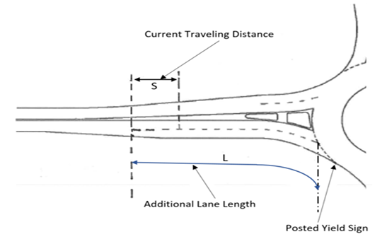 | Figure 1. The diagram of roundabout with the additional lane length of L |
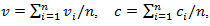
 of vehicle versus to vehicle’s traveling distance
  are shown on Figures 2 and 3.
 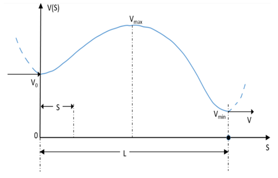 | Figure 2. The diagram of speed of a vehicle when it enters a roundabout without stopping at the “Yield” sign |
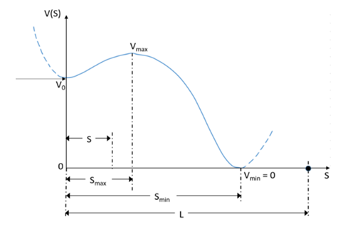 | Figure 3. The diagram of speed of a vehicle when before entering a roundabout it stops behind the “Yield” sign |
 and
and  consequently and a maximum in point
  and it must satisfy to the first order and first degree differential equation having the following general form:
 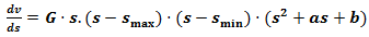 | (1) |
 and
and  have to be positive
  and
and  and relationship between
  and
and  must be as that the radical of expression
  has to be negative, that is
  Integration of this differential equation will give the sixth-degree polynomial function, having the following general form:
  | (2) |
 Because for
  the speed of vehicles is
  , so constant F in equation (2) will have the value
  Therefore equation (2) will obtain the form:
  | (3) |
 in this function also must be positive
  and this function cannot be negative for any values of
  . Based on these conditions as well as on some other additional (initial) conditions, the coefficients
  and
and  of function (3) can be found. Using the system of two equation containing the function (3) and its derivative will allow to solve this problem:
 | (4) |
 | (5) |
 and
and  here some other additional conditions must be used. In our solving problem these additional conditions are interpreted clearly on the diagram, presented on Figure 3. From this diagram it is shown that when vehicle’s traveling distance is
  then speed of vehicle approaches to its maximum value
 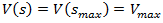 and consequently the rate of changing of speed at that point is
 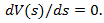 Besides that, when a vehicle travels the distance
  then it stops behind all of vehicles, queening before “Yield” sign. Obviously that location of the stopping spot
  depends on the capacity of the additional lane and it may be relatively close to the entry of that lane or next to the “Yield” sign. Here also for
  vehicle’s speed as well as its rate of changing in respect to
  become zero, that is
 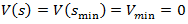 and
and 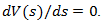 The value of distance when speed of a vehicle again becomes equal to the initial speed
 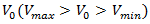 will be denoted as
  However, this traveling distance can be approximated with very high accuracy as the double of distance
  that is
  Graphically it implies that coordinate
  is located approximately in the midpoint between
  and
and  This kind of approximation is equivalent to the consideration that in the interval
  the behavior of the curve
  similar to the second order parabolic function. Applying actual field measurements (for 15 min, half an hour, etc.) of traffic flows in the additional lanes of currently existing roundabouts will allow to perform field data collections to design traffic performance models. These observations, performed on the base of certain conditions, can be used for obtaining statistical dependencies between
  and
and  that is, for finding dependence
  and
and  Analogously there can be found statistical dependencies between
  and
and  , that is
  . Thus, parameters
  and
and  should have statistical interpretation, based on field data collections. If for the given period of time there have been performed
  field measurements then these parameters can be considered as the mean statistical for that period of time, that is
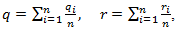
 Obviously, that statistical values of q, r, v and c will strongly depend on the observation period of time, performing during the entire weekday. Mainly the observation periods of week.0day time include early morning, noon (before and after) and early evening. Based on above characterizations of these coefficients they practical values (approximately) can be considered to be laid in the following ranges:
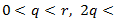
 and
and 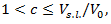 where
where  is the speed limit on the additional lane, having values
  On the base of equations (4) and (5) and above-mentioned conditions a system of equation will be found, satisfying these conditions.
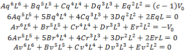 | (6) |
 and is
  belonging to this system of equation can be found as: where
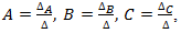
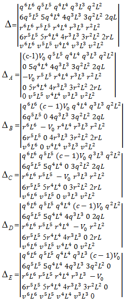 Hence, on the base of above calculations the coefficient
  and
and  will depend on from
  and
and  as well as from the statically observed coefficients
  that is:
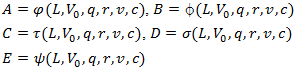 Determining all above coefficients will allow us to find the final version of the general form of the equation (3) representing speed
  of a vehicle verses to its traveling distance
  . Therefore definition of coefficients in equation (3) shows that for the given length of the additional lane
  and for the given value of the initial speed
  the current value of speed
  will depend on from
  and
and  as well as from the statistically observed values of
  and
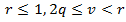
and  Consequently, for the given values of
  and
and  and for different values of statistically defined coefficients
  and
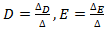
and  here could be obtained whole family of diagrams, illustrated on Figure 4.
 | Figure 4. The family of the analytical diagrams of speed of the vehicles that may take place during the weekday |
 from their traveling distance
  Moreover, for the given values of
  and as well as for the reasonably chosen values of coefficients
  and
and  here can be obtained the similar families of the curves, based just on analytical reasoning. Obviously, that this kind of analytical curves also may have large practical applications in roundabouts entry/exit lines designing. Thus, due to relatedly very short distance of the additional lane and based on this circumstance short-term acceleration-deceleration driving regime of vehicles the dependents of vehicles’ velocity
  from their traveling way
  can be represented through the sixth-degree polynomial function. Therefore, our derived mathematical algorithm will allow roundabout development specialists to find the delay of the vehicles in the availability of the additional entry lane easily. Here it must be noted that currently the HCM only includes control delay, the delay attributable to the control device. The control delay is the necessary time that a driver spends decelerating to a queue, queueing and then waiting for an acceptable gap in the circulating flow while at the front of the queue and accelerating out of the queue. According to our proposed algorithm of kinematics here the current value of braking distance of a vehicle can be found as a difference between the current values of distances
  and
and  As it shown above these distances corresponding to the minimum
  and the maximum
  values of the speed:
  | (7) |
 measurements than statistical average braking distance for that period can be calculated as:
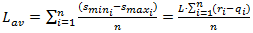 | (8) |
 | (9) |
 | (10) |
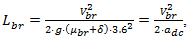
 braking distance (m ≈10, m≈3.28 ft)
 breaking speed (km/h≈3280 ft/h),
 acceleration due to gravity (9.81 m/s2≈32.12 ft/s²),
  mean coefficient of friction,
 roadway grade
 the declaration of vehiclesThe declaration adc of vehicles is defined as:
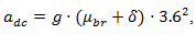 | (11) |
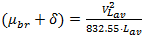 | (12) |
 vehicle, which is required by the National Cooperative Highway Research Program [2]. The point is that HCM for calculations very often recommends using the 95%-percentile vehicle queue length, applied for a given approaching lane. Authors in [39,40] show how the 95th-percentile queue length varies with the degree of saturation of an approach:
 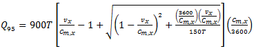 | (13) |
 = 95th-percetile queue, veh;
 flow rate for moment x; veh/h;
 capacity of moment x, veh/h;
  analysis time period, h (T=1 for a 1-h analysis,
  0.25 for a 15-min analysis);
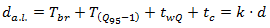
  volume-to-capacity ratio.The volume-to capacity ratio is a comparison of the demand at the roundabout entry to the capacity of the entry and provides a direct assessment of the sufficiency of a given design. For the given lane, that ratio is calculated by dividing the lane’s calculated capacity into its demand flow rate. While the HCM does not define a standard for that ratio, international and domestic experience suggests that value ot that ratio falling in the range 0.85 to 0.90 represents an approximate threshhold for satisfactory operation.Because the capacity of vehicles is one of the key parameters of traffic operations, there are many publications dedicated to this matter. However, Lee Rodegerdts [41] showed U.S.A. universal roundabout capacity model (capacity of moment x) as a function of the circulating flow on the roundabout, follow-up headway, and critical gap through the following general equation.
 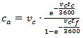 | (14) |
 approach capacity, (veh/h),
  circulating flow rate, (veh/h)
 critical gap, (sec)
  follow-up time, (sec) This equation estimates the capacity of a roundabout’s approach (entry lanes) via input parameters such as circulating conflicting traffic volume
  follow-up time
  and critical gap
  However, earlier studies by Hagring (1996, 1998) found that the critical gap differs between the two entering lanes at a two-lane roundabout. The studies also found that right-turning vehicles in the outer entry lane had significantly smaller critical gaps than those of other turning movements at the same approach. Critical gaps were found to be very similar regardless of which of the two circulating lanes vehicles were entering and it was therefore concluded that both circulating streams impede entering vehicles. Hagring [36,37] related critical gap to the size of the weaving area between two adjacent roundabout approaches with the following equation:
 | (15) |
 = critical gap;
  = length of weaving section;
  = width of weaving section;
  = lane number (outer lane = 1, inner = 2). The circulated flow is calculated for each leg, and the circulating volumes are the sum of all volumes that will conflict with entering vehicles on the subject approach.The average breaking time of
  vehicle is the time that a driver spends decelerating to a queue. Using formulas (8) and (9) we will find vehicle’s average breaking time:
  | (16) |
 vehicle. Application of currently existing high-resolution time-distance measuring video devices (especially designed for queue detectors) will allow roundabout development specialists to solve this problem. Obviously, that before
  vehicle there will be a queue with the
  vehicles, and video devices will be able to measure each
  vehicle’s length
  and its gap
  We also should mention that average lengths of vehicles are distributed by the lengths of passenger cars, light and heavy vehicles. According to American HCM, as a single unit a car, taxi or pickup is used for expressing transportation flow capacity. Cycle and motorcycle are considered as half a car unit. Buses and trucks are considered as 3 care units. Horse-drawn are 4 units, bullock carts 6 units and large bullock cart 8 units. Hence, the length of queue measures in foots or meters, so the length of
  vehicles with their gaps can be expressed as:
 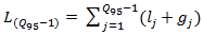 | (17) |
 is the total number of vehicles in queue, defined by formula (17). However, in [3] it is considered the average queue length or number of vehicles (
 vehicles) which can be calculated by Little’s rule:
 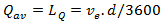 | (18) |
 = entry flow, veh/h; d = average delay, seconds/veh Now let us consider that queue detection technology shows that total merging time of
  vehicles with the roundabout circulating traffic is
  Hence, in that period of time
  vehicle will reach to the end of additional lane or to the “Yield” sign. That time will be considered as a queening time of
  vehicle, and its average speed in queuing will be defined as:
 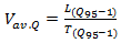 | (19) |
 counts the time for all of
  vehicles, when each of them has to wait for an acceptable gap (sec) to be merged with the circulating flow of roundabout. Obviously that field data collection service will show those waiting times, and they must be differed for each Jth vehicle. So, the total waiting time for al
  can be expressed as
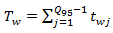 | (20) |
 is the waiting time of the
  vehicle. After queueing, the
  vehicle will wait for an acceptable gap at the front of queue in order to accelerate and exit the queue. Let as consider that the detected value of waiting time of that vehicle is twQ If the length of
  vehicle is lQ then it has to accelerate such way that in the end of the merging cycle it has to be completely located in the circular lane of the roundabout. The speed of that vehicle must be equal (at least) to the roundabout’s circulating speed, showing significant contribution in the merging of vehicles. In [35] it is shown that speed-radius relationship can be calculated by the following formula:
 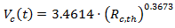 | (21) |
 circulating speed (mi/h)
 aaverage radius of circulating path of through movement (ft). Radius
  can be computed with the equation
 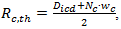 | (22) |
 inscribed circle diameter (ft)
 number of circulating lane(s)
 average width of circulating lane(s) (ft). However, because the speed of vehicles associated with
  can’t remain constant for all of periods of time during the observation, we came up to the conclusion that equation (18) can be modified to obtain the following form:
  | (23) |
 is considered as statistical variable, which can be derived from the observation, completed for the given period of time. The value of
  may lies in the interval,
  where
where  will respond for the minimum value of speed and the
  for the maximum. Obviously, that merging cycle must end at least during the critical gap
  defined by equation (15). Based on these circumstances the acceleration could be found as:
  | (24) |
 vehicle can be estimated as:
  | (25) |
 vehicle, that is
  Thus, we have considered all of components of the control delay of
  vehicle. They are: the time that a driver spends decelerating to a queue
  queueing time
  waiting time
  for an acceptable gap in the circulating flow, and the time
  needed for accelerating and to be out of the queue. Consequently, according to definition of control delay we can confirm that the sum all of these time intervals is equivalent to the such control delay when an additional lane is considered, that is:
 | (26) |
 due to this lane will be less than the control delay
  of the original single lane. Delay
  expressed by the well-known formula, represented in [3]:
 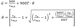 | (27) |
 flow rate for movement x, veh/h
 capacity of movement x, veh/h
 analysis time period,
  for a 15-minute period)
 volume-to-capacity ratio Obviously, that in result of adding a lane the ratio
  must be less than one (1), that is:
  | (28) |
 | (29) |
 represents the desirable or expectable gain of delay, and
  is considered as the control delay of the single-entry lane roundabout. From the above calculations of time components
 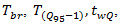 and
and  and also from definition of the control delay
  it can be seen that formula (26) commonly associated with many of parameters of roundabout, such as its additional lane length
  the length of queue
  circulating speed
  average radius
  of circulating path, critical gap
  approaching capacity
  circulating flow rate
  and control delay
  of the single-entry lane. Definition of all these parameters are given above. Therefore, for the given values of
 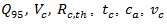 and
and  the value of coefficient
  will depend on the length of the additional lane
  Application of modern technology of data collection as well as computer modeling of formula (26) will allow to find very accurate graphical dependencies of Coefficient
  and delay
  from the additional entry lane length
  Thus, our proposed method will allow us to find the dependence of vehicles’ velocities
  from their traveling distance
  and this method will allow to find the delay due to the length
  of the additional lane. Despite of the method outlined in [16] where for consideration of operational performance of a double-lane roundabout with additional lane length design have been used and analyzed quite complex and inconvenient Lighthill-Whitham-Richards mathematical model, our proposed method is simple and understandable, it is effective and accurate, and considering those advantages it can achieve promising results. Any roundabout design specialist can use our method without demanding significant or specialized expertise in kinematics and mathematical analysis.
 4. Conclusions
- In this paper for calculations of the delay of a vehicle traveling by the additional entry lane of roundabout we proposed to determine the dependence of vehicle’s velocity from its traveling distance. For that purpose, here the combined methods are used, included analytic method and the method of practical data collection. Analytic method has been represented by sixth-degree polynomial function, while data collection is based on the consideration of the time that a driver spends decelerating to queue, queueing time, the number of vehicles in queue, waiting time for an acceptable gap in the circulating flow and the time needed for accelerating out of the queue. For the given value of the length of the additional entry lane and for the given period time of weekdays those above-mentioned combined methods will allow first to find the dependence of vehicle’s velocity from its traveling distance and then vehicle’s delay. After that using the existed/calculated values of the delay of the single-entry lane roundabout the coefficient of the gain of the delay can be found. The ratio of the delay of the additional entry lane to the delay of single-entry lane of roundabout will determine the delay’s gain coefficient. Application of this approach of determination of delay’s gain will lead to obtain the plenty of curves representing the dependence of velocity of vehicle verses to its traveling distance. Our proposed method will allow the roundabout designer to choose the proper length of the additional lane to obtain the desirable delay. Obviously that future improvement of audio-video and time registration technology will create more advanced and precise method of data collection and consequently more accurate generation of the curves representing sixth-degree polynomial functions.
ACKNOWLEDGEMENTS
- The authors are thankful to Dr. Samuel Hammond heading for share with us more detail about his idea regarding to adding of the second-entry lane of the roundabout. The Idea of this subject is presented in his Doctoral Degree Thesis, named by the title: “The effect of Additional Lane Length on Roundabout Delay”.