1. Introduction

The estimation of traffic volumes on a road network is an important issue for a variety of transportation design and planning purposes [1]. A large number of transportation engineering activities require traffic volume estimates. Traffic volumes are generally collected by traffic volume count programs led by state Departments of Transportation (DOTs) and local government agencies. However, these traffic count programs usually take place in urban areas or higher classes of roads. Traffic volumes on rural low-volume roads (defined as less than 400 vehicles per day) are usually ignored [2]. Although low-volume roads serve fewer vehicles than higher classes of roads, such as Interstate highways, they have important impacts on economies for local or regional areas [3, 4]. Low-volume roads serve as links between raw materials and markets. Although traffic volumes may be low on low-volume roads, vehicle loads may be high. In addition, although rural roads carry less than half of nation’s traffic, they account for more than half of the nation’s vehicle fatalities [5]. As a result, low-volume roads typically need reconstruction and improvement. It is significant to estimate traffic volumes on low-volume roads to address planning and safety issues.

The installation of traffic counters on roads is an effective way to estimate traffic volumes. However, it would be prohibitive to install traffic counters on all roads, particularly for rural low-volume roads [6]. An alternative to the traffic counters is to develop a travel demand model to estimate traffic volumes. A four-step travel demand model, including trip generation, trip distribution, mode choice, and trip assignment, is the traditional procedure for transportation forecasting. In a travel demand model, traffic volumes are estimated through the interaction of travel supply and demand [7]. The outputs of a travel demand model include a variety of traffic-related parameters, such as average daily traffic (ADT), travel time, and congestion levels. ADT values from travel demand models are rough estimates based on the input parameters used in models. They can be used in many areas of transportation applications, such as design, forecasting, planning, and policy making [8]. Most state DOTs have developed and implemented four-step travel demand models for large metropolitan areas. However, some of those advanced models are not applicable for most county or rural roads which carry a low ADT. Therefore, a travel demand model that is designed for low-volume roads is needed for local agencies [9].

Apronti and Ksaibati [10] developed a travel demand model to estimate traffic volumes on low-volume roads in Wyoming. Their model included person trips, crop freight trips, and oil freight trips. Their model has a good prediction in most parts of Wyoming (average R square: 0.8) but Northwest Wyoming (R square: 0.6), where Yellowstone and Grand Teton National Parks are located. This study modified Apronti and Ksaibati [10]’s model by incorporating tourism parameters into the model and estimated traffic volumes on low-volume roads in Northwest Wyoming. Tourism is an important part of economy and a significant source of employment [11]. The State of Wyoming is facing a tourism industry development in rural areas. Yellowstone and Grand Teton National Parks are among the top 10 most-visited national parks in U.S. in 2016. Annual visitors to Yellowstone National Park have increased from 3,000,000 before 2000 to more than 4,000,000 in 2017, and annual visitors to Grand Teton National Park have increased from 2,500,000 before 2000 to more than 3,300,000 in 2017 (12). Transportation is a key element in tourism. It is crucial to estimate traffic volumes on rural roads near the parks and improve road network to enhance visitor experience.

2. Literature Review

Many studies have focused on the estimation of traffic volumes and the various factors affecting the values. Zhan et al. developed a hybrid framework to estimate citywide traffic volumes. Their results indicated the effectiveness of the proposed framework in traffic volume estimation [1]. Kwon et al. proposed an algorithm to estimate real-time truck traffic volumes from single loop detectors on Interstate 710 near Long Beach, California. The algorithm was able to capture the daily patterns of truck traffic volumes and mean effective vehicle length with only 5.7% error [13]. In addition to urban areas and Interstate highways, the issues of traffic volumes on low-volume roads have also been addressed in some research. Sharma et al. applied artificial neural networks to estimate average annual daily traffic (AADT) on low-volume rural roads in Alberta, Canada. They found a number of advantages of the neural network approach in AADT estimation compared to the traditional approach [4]. Karlaftis and Golias developed a statistical methodology to assess the relationship between rural road geometric characteristics and traffic volumes on rural roadway accident rates. The methodology they developed allowed for the explicit prediction of accident rates on rural roads [14]. Raja et al. developed a linear regression model to estimate AADT on low-volume roads for 12 counties in Alabama. Their research concluded that the linear regression model can be used to estimate AADT on low-volume roads for future application [15].

A number of factors can affect traffic volumes. Demographic data, including population, household, and employment, are usually used in travel demand model [16]. To improve the model prediction accuracy, some other factors were also included in the previously developed models. In addition to demographic data, Saha and Fricker used some economic factors, such as gasoline price, consumer price index (CPI), and gross national product (GNP) to develop models for rural traffic forecasting [17]. Tourism-related traffic volume is also a critical part in regional transportation planning. Many states’ travel demand models considered the impact of tourism. The Florida DOT District Five office (covering the Orlando region) developed a model to provide more accurate forecasts of tourism travel to central Florida. The goal was to produce more policy-sensitive forecasts to inform ongoing transportation planning efforts. The model covered more detailed dynamics of trip generation and allocation by visitors to a destination. The model included three tourist trip purposes: Disney tourist (Disney to and from hotel), Disney resident (Disney to and from homes in the Orlando area), and Disney external/internal (Disney to and from external stations). Additional attraction-oriented trip generation was also considered for Universal Studios and Orlando International Airport. The study was successfully completed by focusing on improving the highway network and forecasting traffic flow [18]. By using a more robust set of explanatory variables in model development, the model will better predict the future traffic patterns.

There is a growing need for incorporating tourism into travel demand models for transportation planning [19]. One element making this the time to consider tourism in transportation planning is the growing number of visitors to the U.S. national parks. There is a wide range of issues need to be addressed at the intersection of tourism travel and the transportation facilities currently available to carry tourists [20]. Another element is the development of transportation and travel modeling software. As geographic information system (GIS) and related software has been widely used in research and practice, more comprehensive travel models have been developed [21]. A final element is the rapid growth of many urban and suburban communities extending to the areas once known as rural, which has changed traffic patterns and local economies [22]. Therefore, an inexpensive and effective means of estimating traffic volumes on the state’s low-volume roads is highly desirable [23]. It will assist government and travel agencies in transportation decision making.

3. Methodology

Seven counties in Northwest Wyoming were selected as the study area for developing models to estimate ADT. Figure 1 shows the study area. Northwest Wyoming is home to Yellowstone and Grand Teton National Parks as well as some other popular tourist destinations, such as Jackson and Lander. This region was analyzed in this study since this region attracts many tourists throughout the year. Both Yellowstone and Grand Teton National Parks have multiple entrances. Figure 2 presents the park entrances included in this study. The traffic volumes at these entrances were analyzed since visitors who go through these entrances will use roads in Wyoming.

Figure 1. Study Area

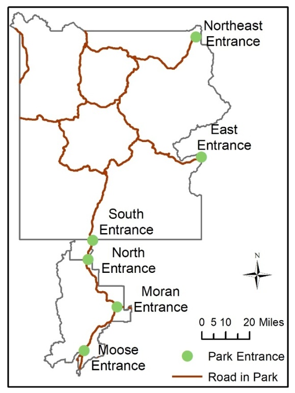Figure 2. Park Entrances Included in the Study

3.1. Tourism Seasonality

Seasonality is a key element in tourism industry. Seasonal patterns of tourism travel demand create overcrowding traffic at certain times. The analysis of seasonality in tourism demand helps to improve the accuracy of modeling results [24]. Based on the monthly visitation data from the U.S. National Park Service (NPS), the year was divided into peak season and off-peak season. Figure 3 shows average monthly ADT at all six park entrances in 2014. The year of 2014 park visitation data was used in this study since the actual traffic count data used for model validation was mostly obtained in the summer of 2014. Based on the monthly traffic count, peak season is defined as May through October, and off-peak season is defined as November through April.

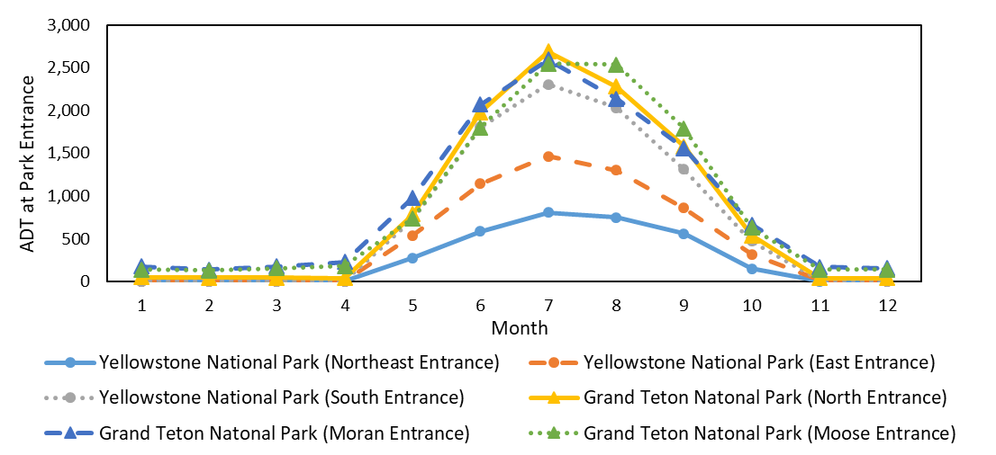Figure 3. ADT at Park Entrance

3.2. Travel Demand Model

A four-step travel demand model, including trip generation, trip distribution, mode choice, and trip assignment, was developed by Citilabs’ Cube software in this study. Esri’s ArcGIS software was also used to perform some GIS analysis. Three ArcGIS shape files: road network, transportation analysis zones (TAZs), and actual traffic counts were used in the procedure of model development and model validation. Many parameters need to be considered for model development, primarily including socioeconomic data, land use types, and roadway networks. Socioeconomic and land use data are usually arranged into geographic units to design TAZs [19]. TAZs are used to create trip generation equations. The design of TAZs in this study was completed with GIS technology. Figure 4 shows the TAZs and road network in the study area. There are 513 TAZs in the study area. The boundaries of the TAZs frequently cross city and county boundaries.

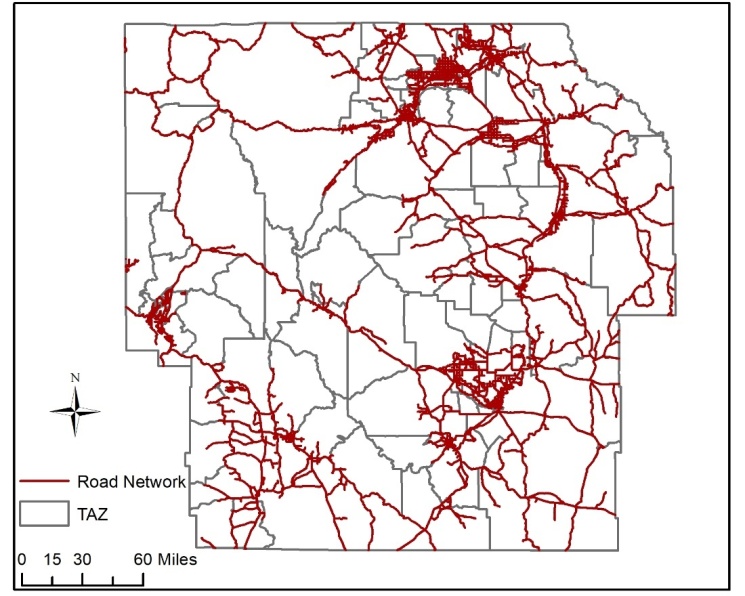Figure 4. TAZs and Road Network

3.2.1. Trip Generation

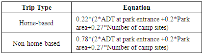
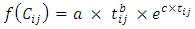
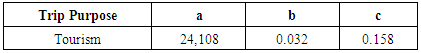
The trip generation procedure defines the number of total daily trips at the TAZ level. This procedure splits each trip into a production and an attraction [7]. However, for tourism trips, only attraction was considered in this study since productions and attractions are defined by the land use and tourism/recreation land use is defined as attraction [25]. The trip attraction model provides a measure of relative attractiveness of tourism destinations as a function of socio-economic and land use variables. Home-based trips (trips with both ends in the study area) and non-home-based trips (trips with one end outside the study area) were analyzed separately in the model. Three tourism-related parameters, including ADT at park entrances, park area, and number of campsites in park, were selected to determine trip rates. The selection of these parameters was based on their significance, sensitivity, and forecastability, which are recommended by the Trip Generation Manual [25]. Table 1 lists the trip generation equations for each trip type. The constants (2, 0.2, and 0.27) before each parameters were obtained from the Trip Generation Manual [25]. The constants of 0.22 and 0.78 indicate that 22% of total tourism trips were generated by visitors from Wyoming and 78% of total tourism trips were generated by visitors from other states or countries. Those ratios were obtained from the NPS visitor survey [12].

Table 1. Trip Generation Equations

3.2.2. Trip Distribution

In the procedure of trip distribution, the trips generated in each zone in trip generation procedure are then distributed to all other zones based on the choice of destination [7]. This procedure creates a trip matrix that lists the number of trips going from each origin to each destination. Two main methods are usually used to distribute trips among destinations: gravity model and growth factor model [26]. This study applied the gravity model method, derived from Newton’s fundamental law of attraction, to distribute trips from each origin into distinct destinations. The gravity model is expressed as follows:

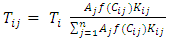(1)

where:

T_ij = trips from i to j;

T_i = trips produced in zone i;

A_j = trips attracted to zone j;

f (C_ij) = friction factor related to travel time;

K_ij = optional trip distribution calibration factor.

The friction factor is expressed as follows:

(2)

where:

a, b, c = constants listed in Table 2;

t_ij = travel time between zone i and j.

The constants of a, b, and c were obtained from the Trip Generation Manual (25). Travel time was calculated by dividing total distance between zone i and j by posted speed limit. For unpaved roads, a speed of 10 mph was assigned in the model.

Table 2. Coefficients Used in Equation (2)

The optional calibration factor, K_ij, was not considered in this model, since it has not been completed identified for tourism. Previous research indicated that this factor is related to some socio-economic parameters such as income and occupation (7). Since there is no available data for tourists’ income and occupation, this research ignored calibration factor in the gravity model.

3.2.3. Mode Choice

The procedure of mode choice determines the means of travelling. Only the mode of personal vehicle is considered in this study since other travel modes, such as public transportation, are not significantly represented in the study area. In this procedure, average vehicle occupancies were used to create the trip matrix of personal vehicle trips. In this study, the average auto-occupancy rate (persons/vehicle) is 3.04, which was obtained from the NPS visitor survey [12].

3.2.4. Trip Assignment

The trip assignment procedure allocates a given set of trip interchanges to the specified transportation network. In this procedure, the traffic volumes on each road segment will be estimated, and the travel patterns will be analyzed [26]. This procedure calculates the shortest path from each zone to all the other zones. The assigned number of trips are compared to the capacity of the road to see if it is congested. If a road is congested the trip routes are changed to result in a longer travel time on that road. The whole process is repeated several times until there is an equilibrium between travel demand and travel supply.

4. Results

4.1. Model Outputs

The visitation data in peak season of 2014 was input into the travel demand model. Figure 5 shows the spatial distribution of low-volume roads (ADT ≤ 400) and non-low-volume roads within the study area. Figure 6 presents the estimated ADT without and with tourism. It identifies road segments which have higher traffic volume due to tourism activities. It can be seen from Figure 6b that after incorporating tourism into the model, traffic volume has increased on the low-volume roads near the parks.

4.2. Model Validation

Validation of the model results to locations that have actual traffic counts is necessary so that it can be shown that the model is within expected ranges. In validating the travel demand model, traffic volumes generated by the model were compiled and compared to actual traffic volumes on 76 selected low-volume roads in the study area. Figure 7 show the locations of actual traffic counters for model validation. Without tourism, the predicted ADT and the actual ADT resulted in an R square value of 0.60. After incorporating tourism, the predicted ADT and the actual ADT resulted in an R square value of 0.88. Although the tourism-based travel demand model well predicted ADT, there are some factors that should be considered in using the model and its results:

1. The model estimates are not applicable to urban roads including low-volume roads that leads directly to or within an urban area.

2. The model estimates are not applicable to Interstates and State highways.

3. The model estimates are for the higher summer traffic volumes only, since visitation data from peak season (May to October) was input into the model.

4. Not all access roads within TAZs are captured by the model. Some minor access roads within a TAZ may be represented by a single centroid connector. The estimated volume for any of the access roads within such a TAZ will therefore be determined as being less than or equal to the traffic volume on that centroid connector.

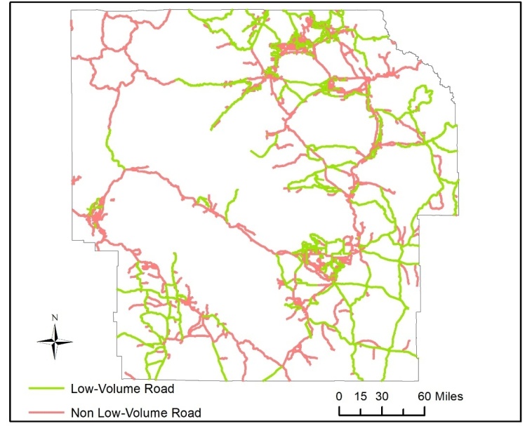Figure 5. Low-Volume Road vs. Non Low-Volume Road

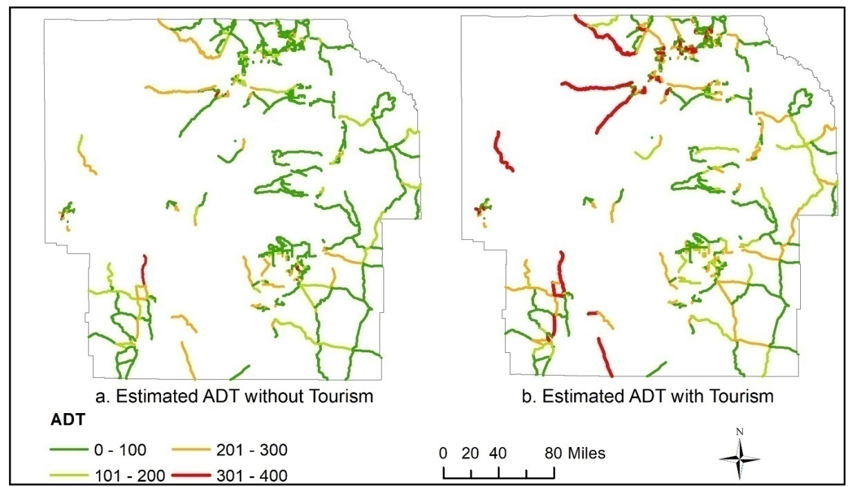Figure 6. Estimated ADT without vs. with Tourism

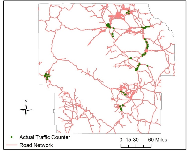Figure 7. Locations of Actual Traffic Counters for Model Validation

5. Conclusions and Recommendations

Tourism travel is a significant portion of the total travels in Northwest Wyoming and low-volume roads provide links to some popular recreational facilities. This study presented a method for estimating traffic volumes on low-volume roads due to tourism activities. In this study, a tourism-based travel demand model was developed to estimate ADT in Northwest Wyoming. Actual traffic counts were used for calibration purposes. It has been shown that tourism can be incorporated into a traditional four-step travel demand model to predict tourism-related ADT on the local road network. This data can then be compared to actual traffic data to locate sites that may have underrepresented traffic flows. The results from the model proved the existence of high traffic volumes in rural area. It can be concluded from this study that the low-volume roads near Yellowstone National Park will experience traffic volume increase due to an increase in tourism trips. While this work looked specifically tourism trips near Yellowstone National Park, the method could be applied to any trip type that has known origin and destination information. The model results can be applied in a variety of transportation designs and planning.

The conclusions of this study are as follows:

1. A travel demand model is useful and practical for estimating traffic volumes on low-volume roads. A variety of tourism-related parameters, including ADT at park entrances, park area, and number of campsites in park were considered in trip generation to estimate the number of trips.

2. Compared to the actual traffic counts, the travel demand model has an 88% prediction accuracy after incorporating tourism into the model, which well captures the traffic flows on low-volume roads near tourism destinations. The local roads with high traffic volumes should be given priority in transportation planning and maintenance.

3. The results of this study indicated that travel demand model is capable to work well with a variety of tourism data sets and can be used to predict traffic volumes in future.

Rural tourism is a significant part of global tourism industry. All regions around the world have shown increasing tourists in rural areas, with the fastest growth in Europe, Asia, and Americans. This study shows the significance of capturing the tourism-related traffic volumes in rural areas for transportation planning and maintenance. The tourism-based model can be easily incorporated into the existing statewide travel demand model and used for future tourism travel demand prediction. This study also adds to the existing knowledge on the estimation of traffic volumes by travel demand model in rural areas. Previous studies mainly focused on estimating traffic volumes in urban areas and Interstate highways. The model developed in this study can be used to estimate ADT in the rural areas where tourism is a major generator of traffic flow on low-volume roads and not enough traffic counters are installed. The model is recommended to update based on the updated census data from the U.S. Census Bureau and the visitation data from the NPS. The model developed in this study is recommended to be applied by government and tourism agencies in other states or countries when census data and tourism visitation data are available.

ACKNOWLEDGEMENTS

The Wyoming Department of Transportation (WYDOT) and the Mountain-Plains Consortium are acknowledged for funding this study. The Wyoming Technology Transfer Center is also acknowledged for facilitating this study by making available resources and providing relevant training. All figures, tables, and equations listed in this paper are work in progress and they will be published in a WYDOT report at the conclusion of this study.