Punyaanek Srisurin 1, Amarjit Singh 2
1Department of Civil, Environmental and Architectural Engineering, The University of Kansas, Lawrence, KS, USA
2Department of Civil and Environmental Engineering, University of Hawaii at Manoa, Honolulu, HI, USA
Correspondence to: Amarjit Singh , Department of Civil and Environmental Engineering, University of Hawaii at Manoa, Honolulu, HI, USA.
| Email: |  |
Copyright © 2017 Scientific & Academic Publishing. All Rights Reserved.
This work is licensed under the Creative Commons Attribution International License (CC BY).
http://creativecommons.org/licenses/by/4.0/

Abstract
This study aims to determine the best resolution to minimize the count of idling automobiles at the intersection of McCully Street and Kapiolani Boulevard. The optimal traffic signal timing for traffic flow during the evening rush-hour commute, 6 p.m. to 8 p.m., was examined in all movements. The U.S. Federal Highway Administration regulation for standard walking speed, four feet per second, was considered to ensure the safety of pedestrians. Traffic signal durations were decided using linear programming, based on the average number of idling automobiles, existing pedestrian crossing signal timing, and the rate of vehicular arrivals to the intersection. Vehicular arrivals were measured for each movement in order to calculate the total number of automobiles waiting for the green indication. Automobiles at this intersection are permitted to make right turns on red, as long as it is safe for them to proceed, given by an absence of pedestrians at the crosswalk, and no other vehicles at the intersection. Because the “right on red” traffic management policy applies to this intersection, the study focuses on the number of automobiles waiting to turn left or making through movement. The results show that the optimal effective green time for vehicles making through movement on McCully Street should be twenty-three seconds (36.1% shorter), while the optimal effective green time for vehicles making through movement on Kapiolani Boulevard should be twenty seconds (58.3% shorter). Besides, the optimal effective green time for vehicles making left turn on either street should have an effective green time of twelve seconds (one increases by 50%, while the other reduces by 33%). Red indications should reduce by 24.2% on the through movements. The queue lengths at the intersection are reduced in a range from 24.2% - 46.1%, proportionally with the red times reduction. This just means that the mobility at the intersection increases, thereby minimizing the overall queue length. In conclusion, the longer green time assignment on the movements that possess relatively higher arrival rates does not necessarily mean that the number of vehicles queuing at an intersection is reduced by as much as the shorter red time on those movements. Also, the longer green times may create an excessively long cycle length that generates longer queues on the other movements.
Keywords:
LINDO, Linear programming, Peak period, Queue length, Traffic signal, Vehicle flow, Pedestrian walking speed, Green time, Red time, Signalized intersection, Signal optimization
Cite this paper: Punyaanek Srisurin , Amarjit Singh , Optimal Signal Plan for Minimizing Queue Lengths at a Congested Intersection, International Journal of Traffic and Transportation Engineering, Vol. 6 No. 3, 2017, pp. 53-63. doi: 10.5923/j.ijtte.20170603.02.
1. Introduction
Traffic signals at intersections exist to keep traffic safe, both for automotive and pedestrian traffic. Intersections pose the greatest safety risk to traffic, as this is where traffic meets that travels in cross directions. The duration of traffic signals must be manipulated in order to optimize the safe flow of traffic through the intersection. Moreover, optimizing traffic signals to reduce the number of idling vehicles can also benefit the reduction in fuel consumption and emissions as well [10, 12]. Typically, Webster’s method is widely applied to determine the optimal cycle length based on delays. However, at high saturation flows, the cycle length could be overestimated [14]. Although, in most cases, delay based approaches are more common to determine optimal signal plan [11], this study opts to use an alternate approach by considering queue length as the main measure to tackle traffic congestion at an intersection since congestion is primarily caused by the development of long queues [9]. Considering the rate of traffic flow will vary throughout the day, and coupled with varying widths of crosswalks, the vehicular and pedestrian traffic flow [8] at intersections can be enhanced by using non-standard traffic signal durations. The intersection of Kapiolani Boulevard and McCully Street in Honolulu was chosen for examination in order to determine if the traffic flow through this intersection could be optimized during the evening rush hour, which is from 6 p.m. until 8 p.m., using the number of idling vehicles at this intersection as an indication of existing traffic demand. The signal control at the intersection applies a pretimed control of 110-second cycle length. The study solves the problem by simplifying the traffic system at the Kapiolani - McCully intersection by utilizing linear programming to examine the existing conditions; as such, the fluctuations of vehicular arrival rates from all directions were omitted. Alternatively, average vehicular arrival rates during the two-hour p.m. peak were used to determine the total number of vehicles idling at the intersection. Besides, the study assumes the intersection is an isolated system that the consequences of traffic flow from this intersection to the others, and vice versa, are neglected. At the intersection of Kapiolani and McCully, traffic directions may be characterized into four directions as follows: travelling eastbound or westbound on Kapiolani Boulevard, and travelling northbound or southbound on McCully Street. Each general direction can be further categorized into three groups based on intended movement: turning left, turning right and making through movement. Given that automobiles are permitted to make right turn on red indications; thus, only left turn and through movement traffic are focused in this study. Consequently, eight movements are considered in this study.
1.1. Signalized Intersection
Prior to drilling into the details of this study, discussions on the nature of the Kapiolani-McCully signalized intersection shall be presented. Kapiolani Boulevard consists of seven lanes on both sides of the intersection. Through movements, for both sides, are allowed on the three rightmost lanes. For each side, the left turn from Kapiolani Boulevard to McCully Street is allowed on the middle lane, while the other three lanes on the left are allowed for vehicles from the other directions to occupy. Comparably, McCully Street consists of five lanes on the north, and six lanes on the south. The rightmost lane on the south is only available for right turn; thus, it is neglected from the study because vehicles occupying that lane flow relatively freely. Through movements are allowed on the two rightmost lanes for north McCully, while the second and third rightmost lanes on south McCully are allowed for the same purpose. The left turns from McCully Street to Kapiolani Boulevard are allowed on the third and fourth rightmost lanes for vehicles heading from north McCully and south McCully, respectively. The other two lanes on the left are allowed for vehicles from the other directions to occupy. The pretimed signal control of 110-second cycle length is adopted for the intersection during the study period. Besides, all-red times are assigned zero for all phases at the intersection in this study. In addition, the startup delays at the beginning of the green indication and the clearance delays are assumed zero, and so are neglected in the models. Subsequently, the term “green time” in this study exclusively means the effective green time, composed of green time and yellow time. On the other hand, the term “red time” in this study accordingly means effective red time itself.The signal control at the intersection consists of four phases, in which each pair of movements are activated at a time, while the other six movements simultaneously consolidate vehicles in their lanes. When a green time of any pair of given movements ends, the vehicles on those lanes are signaled to stop, and vehicles on the next pair of movements are signaled to proceed. The system runs in this manner until all four phases are activated, starting from McCully through movement and followed by McCully left turn; Kapiolani left turn; and Kapiolani through movement, in that order, to complete a cycle. Figure 1 illustrates the three-letter notations for vehicle arrival rate variables, which are further explained in the nomenclature section. Their effective green times are denoted by T1, T2, T3, and T4.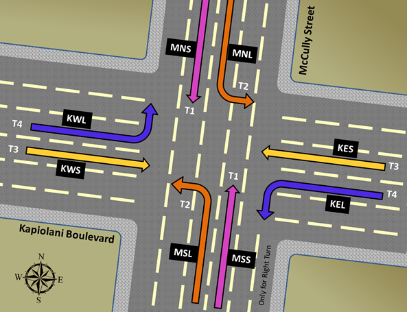 | Figure 1. Kapiolani – McCully intersection layout |
2. The Linear Programming Model
2.1. Development of the Objective Function
The goal is to reduce to the minimum the number of automobiles idling at the intersection, considering the typical arrival rates of vehicles, and existing effective green durations for vehicles to turn left or making through movement. In order to approximate the number of idling vehicles, the study multiplied the arrival rate of automobiles travelling in each movement by the duration of the corresponding red time assigned to the affected traffic lanes. Put another way, queue length for each movement may be calculated by multiplying the rate of arrival by the corresponding idle time. As an example, vehicles turning left from McCully Street onto Kapiolani Boulevard are in lane MSL (Figure 1), and the duration of the corresponding green signal is labelled as T2. The duration of this cycle is T2+T1+T4+T3, in that order. Thus, the resultant queue length is MSL x (T1+T4+T3). Therefore, the objective function is: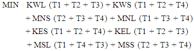 | (1) |
To explain, when a green time of any pair of given movements ends, the pair of movements start consolidating vehicles during its red time, which equals the combination of the other three effective green durations. Then the number of idling vehicles for each movement is determined by multiplying its arrival rate by the corresponding red time. For instance, the pair of north McCully and south McCully through-movement lanes consolidate vehicles for the same amount of time, which equals T2 + T3 + T4. Thus, the pair of those movements consolidate the number of vehicles of {MNS (T2 + T3 + T4) + MSS (T2 + T3 + T4)} in a cycle. Likewise, the pair of eastbound Kapiolani and westbound Kapiolani through-movement lanes consolidate the number of vehicles of {KES (T1 + T2 + T4) + KWS (T1 + T2 + T4)} in the cycle. The number of vehicles consolidated by the pair of north McCully and south McCully left-turn lanes is {MNL (T1 + T3 + T4) + MSL (T1 + T3 + T4)}, while the number of vehicles consolidated by the pair of eastbound Kapiolani and westbound Kapiolani left-turn lanes is {KEL (T1 + T2 + T3) + KWL (T1 + T2 + T3)}. The combination of these numbers of vehicles, which is aimed to minimize by the study, represents the total number of vehicles that idle at the intersection in one cycle.
2.2. Identification of Constraints
Effective green times should be maximized for those traffic lanes having the relatively higher rates of traffic flow. Nonetheless, three factors reduce the duration of “proceed time” to the lanes, regardless of traffic volume. The rate of vehicular traffic in other lanes, and the number of automobiles idling while waiting to proceed must also be considered. The third factor, which is of paramount importance, is pedestrian safety.
2.2.1. Constraints of Pedestrians
The U.S. Federal Highway Administration has established an average pedestrian speed of four feet per second in order to calculate pedestrian “proceed time” [2]. The two crosswalks on Kapiolani Boulevard at the intersection with McCully Street have a length of roughly ninety feet. Conversely, the two crosswalks on McCully Street at the intersection with Kapiolani Boulevard have differing lengths: the northern crosswalk is merely sixty feet, while the southern crosswalk has a length of eighty feet, as shown in Figure 2. In order to adequately address safety concerns, the study uses the longest crosswalk on each street in order to establish a safe duration of the green times given to pedestrians. As a result, lengths of ninety and eighty feet are used for Kapiolani and McCully, respectively. 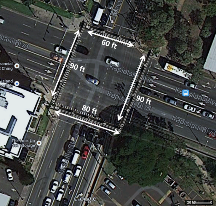 | Figure 2. A top view of the Kapiolani – McCully intersection presenting crosswalk lengths (Source: Google Maps) |
The minimum green times, corresponding to pedestrian safety, are determined by dividing the road widths by the suggested pedestrian walking speed of 4 feet per second. Due to unavailability for pedestrians to cross the streets during the left turns, only T1 and T3, which are effective green times for through movements, are considered to determine safe crosswalk countdown times. | (2) |
 | (3) |
2.2.2. Constraints Related to Queue Length
In order to set the limit of the maximum number of vehicles waiting to make turns for each movement, constraints related to queue length for all the considered eight turns are set in this study. For the sake of optimizing vehicular flow through the intersection, a maximum of ten idling vehicles was used as a limiting factor. As a result, the maximum number of vehicles in each lane waiting for a green indication is: 10 x number of lanes available for traffic to proceed in each movement. Consequently, the following constraints are established to control queue lengths at the intersection:Kapiolani Blvd. (eastbound) contains 3 lanes; thus, | (4) |
Kapiolani Blvd. (westbound) contains 3 lanes; thus,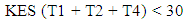 | (5) |
McCully Street (southbound) contains 2 lanes; thus,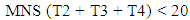 | (6) |
McCully Street (northbound) contains 2 lanes; thus,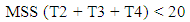 | (7) |
Kapiolani Blvd. (west) to McCully Street (north) contains 1 lane; thus, | (8) |
Kapiolani Blvd. (east) to McCully Street (south) contains 1 lane; thus, | (9) |
McCully Street (north) to Kapiolani Blvd. (east) to contains 1 lane; thus,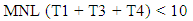 | (10) |
McCully Street (south) to Kapiolani Blvd. (west) to contains 1 lane; thus,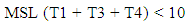 | (11) |
2.2.3. Constraints Related to Vehicle Flow
The duration of effective green times for vehicles turning left was not restricted by the crosswalk factor due to the crosswalks effectively being “off limits” to pedestrians while vehicular traffic was permitted to turn left. As a result, constraints to automotive flow were established for all vehicles making left turn and through movement. For automobiles making through movement, the absolute distance for the final vehicle to proceed across the intersection was the width of the perpendicular road, with an additional length of ten vehicles. Additionally, the length of automobiles ranged from 16.4 feet for a standard sized sedan, which actually can be categorized into 5 sizes itself, to 17.6 feet for a luxury vehicle [6]. As a result, this study applied a median vehicle length, between a standard sedan and a luxury vehicle, of 17 feet in order to calculate safety factors. This produced an estimated travel distance of (90 + (17x10) feet = 260 feet for vehicles proceeding through on McCully Street, as shown in Figure 3, while the distance for vehicles proceeding through on Kapiolani Boulevard was (80 + (17x10) feet = 250 feet. 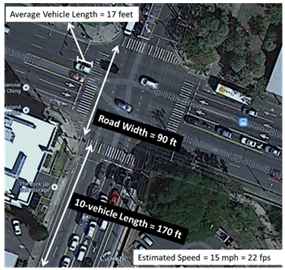 | Figure 3. A schematic shows longest distance for a through movement on McCully (Source: Google Maps) |
The factor of vehicles having different turning radius owing to their size and power must also be taken into consideration. The study assumes that each curve distance can be approximated by a quarter of an ellipse perimeter, in which the corresponding major radius (a) and minor radius (b) are taken into account.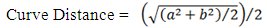 | (12) |
For example, the curve distance for a vehicle taking south McCully and making left turn to Kapiolani Boulevard is approximated by major radius and minor radius of 60 feet and 40 feet, respectively. Thus, the corresponding curve distance is estimated to be 80 feet, as shown in Figure 4. The distances of all the left-turn curves are summarized in Table 1. 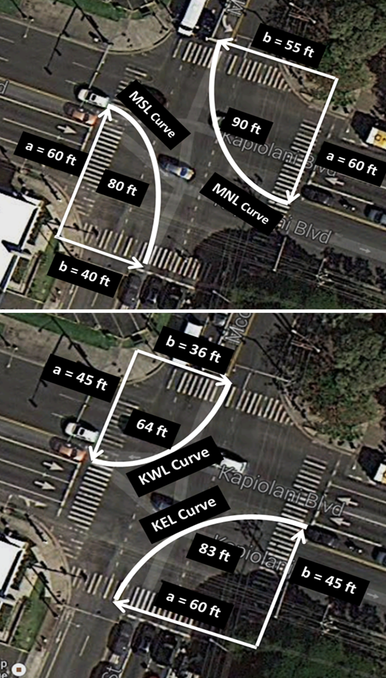 | Figure 4. Schematic shows turning radiuses and the corresponding curve distances for left turns at the intersection (Source: Google Maps) |
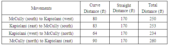 | Table 1. Curve distance, straight distance, and total travel distance for the last vehicle of each left turn |
In accordance with city and county ordinances in Honolulu [1], the speed limit is twenty-five miles per hour unless otherwise posted; however, a vehicle idling at an intersection starts from a speed of zero when the signal turns green. In addition, vehicles making turns – going either right or left – tend to travel slower than vehicles making through movement. In order to provide a realistic speed of vehicles turning left through this intersection, a speed of 15 miles per hour (22 fps) was applied. The minimum green time under the vehicle flow constraint for each through movement is determined by dividing the total distance for the last car to travel across the intersection by 15 mph – the speed limit. Correspondingly, the vehicle flow constraint for each left turn estimates the minimum green time by adopting the 15 mph speed to divide the combination of 10 vehicle lengths plus the curve length. The longer duration for each pair of movements, governed by the same green time, is proposed in the model. Consequently, the vehicle flow constraints are established as follows:Kapiolani Boulevard (eastbound and westbound) 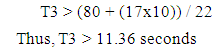 | (13) |
McCully Street (northbound and southbound) 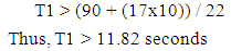 | (14) |
Kapiolani Boulevard (west) to McCully Street (north) 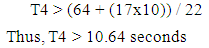 | (15) |
Kapiolani Boulevard (east) to McCully Street (south) 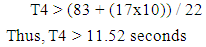 | (16) |
McCully Street (north) to Kapiolani Boulevard (east) 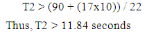 | (17) |
McCully Street (south) to Kapiolani Boulevard (west) 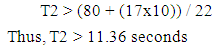 | (18) |
2.3. Data Collection
Raw data was collected to discern the rate of arrival of vehicles to the intersection. The authors randomly observed vehicle arrivals during the 6 p.m. to 8 p.m. evening commute on various days. Given the existing traffic signal patterns at the intersection, the number of arriving vehicles was recorded, and the vehicles were assigned designations specifying the lane in which they arrived at the intersection, their intended direction of travel, and the existing cycle of T1+T2+T3+T4. The vehicle arrival rate of each movement can be ascertained by dividing the total arrivals by the duration of data collection time. For the purposes of this study, a sample size was considered sufficient when a minimum of thirty observations were recorded. The raw data of the number of arriving vehicles during the two-minute period is shown in Table 2. The statistical analysis shows that the vehicle arrival rates are: KEL = 0.05944 (veh/s), KES = 0.22056 (veh/s), MSL = 0.03611 (veh/s), MSS = 0.09639 (veh/s), KWS = 0.26833 (veh/s), KWL = 0.03000 (veh/s), MNS = 0.08278 (veh/s), and MNL = 0.01389 (veh/s).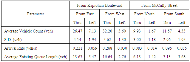 | Table 2. Vehicle arrival rates at the intersection during the two-minute data collection period |
3. The Linear Programming Code
The study utilized linear programming, and used LINDO as a diagnostic tool. The authors acknowledge that stochastic simulation processes would have been more accurate since fluctuations of vehicle arrival rates are neglected when linear programming is adopted as the study tool. However, the study opted to scope merely on the two-hour p.m. peak, in which the vehicle arrival rates at the intersection are perceived to be consistently high; therefore, the fluctuations were assumed to have less impact and negligible in this study since the short time interval of similar traffic demand was segmented [15]. The full LINDO programming code used, which includes the objective function, constraints for queue lengths, constraints for vehicle flow rates, and crosswalk countdown time constraints, is now presented in Figure 5.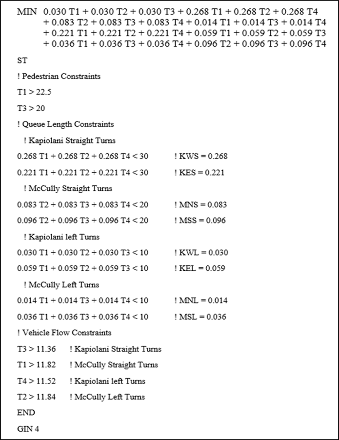 | Figure 5. LINDO code used to minimalize the amount of idling vehicles |
According to the LINDO programming code, each constraint used in the code is adapted from the relevant equation in order to make it compatible to the syntax of the program. To say, the only variables allowed in each constraint must be the ones that appear in the objective function, while the use of parenthesis is invalid in LINDO syntax. Thus, the other variables need to be substituted with specific numbers, and the equation must be decomposed [13]. To illustrate, according to section 2.2.2, the queue length constraint for the eastbound Kapiolani Boulevard through movement is written as KWS (T1 + T2 + T4) < 30, which can be interpreted that the number of eastbound vehicles consolidated on the Kapiolani Boulevard during its red indication is limited to 30 vehicles, where KWS is its vehicle arrival rate. Based on the syntax of LINDO, KWS needs to be substituted with a known number; thus, it becomes 0.268 veh/s, according to its value in Table 2. Thereafter, the constraint becomes 0.268 (T1 + T2 + T4) < 30. Consequently, it can be written as a syntactically correct LINDO constraint as: 0.268 T1 + 0.268 T2 + 0.268 T4 < 30.
4. Results
The study concludes that the optimal effective green time for through movements on McCully street should be twenty-three seconds (T1 = 23); an effective green time of twenty seconds for through movement on Kapiolani Boulevard (T3 = 20); and finds that the optimal effective green time for all left turns should be twelve seconds (T2 and T4 = 12). This time is optimal for minimizing the quantity of vehicles idling at the intersection, and gives consideration to pedestrian safety as well as the number of automobiles waiting to proceed. Compared to existing conditions at the intersection, T2 would see a slight increase in effective green time, 4 seconds; conversely, all other times would be decreased significantly. T1’s duration would be 13 seconds shorter, while T3’s duration would be 28 seconds shorter. Furthermore, T4’s duration would be reduced from the existing 18 seconds to roughly 12 seconds. Besides, T2’s duration is suggested to increase from the existing 8 seconds to 12 seconds, which is a 50% increase, as presented in Table 3. Consequently, all these splits sum up a cycle length of 67 seconds, which is 43 seconds shorter than the existing cycle length. However, it must be noted that the number of idling vehicles programmed into LINDO was 38.5, while the observed average number of vehicles idling at the intersection during 6 p.m. to 8 p.m. was 56.9 vehicles.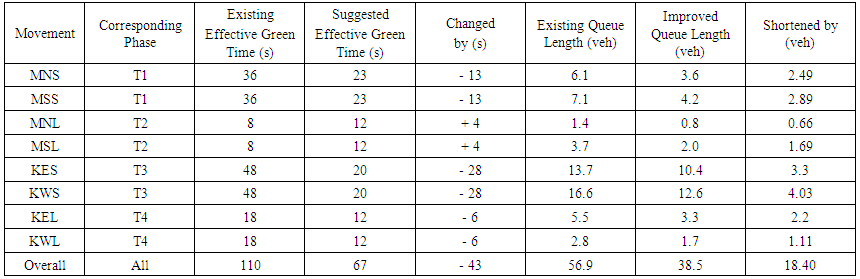 | Table 3. Queue lengths comparison between the existing and suggested signal systems |
The results from LINDO, displaying the selected constraints from the linear programming code that optimize the objective function, is presented in Table 4. In addition, slack variables, which indicate the margins between the optimal signals that optimize the objective function and the signal that satisfy each constraint [5], are illustrated in Table 5.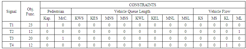 | Table 4. Results of Linear Programming |
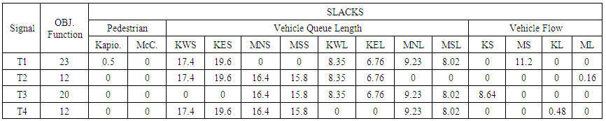 | Table 5. Slack Results from LINDO |
Were the revised signal control to be applied to the Kapiolani Boulevard and McCully Street intersection, the study finds that the number of idling automobiles would be reduced by more than one-third, a reduction of 18.4 vehicles, or 32.3%. The average backlog of traffic under both the current and the suggested green timing durations are illustrated in Figure 6.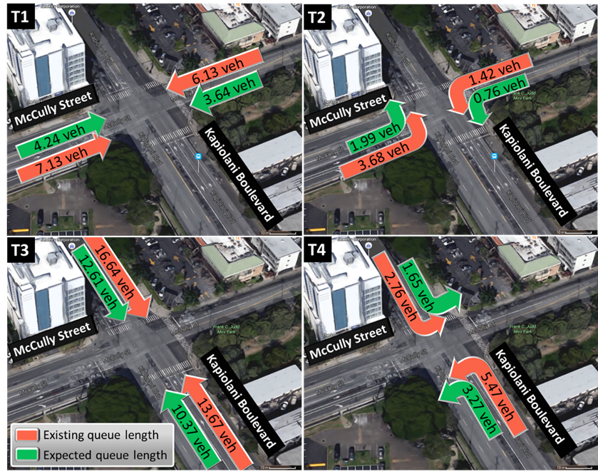 | Figure 6. The existing and the expected average queue lengths at the intersection when the suggested signal control is applied (Source: Google Maps) |
5. Queue-Length Based and Traditional Delay Based Cycle Length Optimization Approaches
Typically, the approaches to mainstream optimal signal planning are performed on the basis of delay minimization, whereas our study uses an alternate approach of considering the minimization of queue lengths under the presence of existing constraints at the intersection in order to amplify the significance of red times on queue lengths, which has not been documented in previous studies. Besides, we assumed that the startup and clearance delays (L) are absent in this study to spotlight the impact of red times on queue lengths, even though they are the main input measures to the delay-based approaches. On the other hand, there are no such constraints as pedestrians and vehicle queue lengths taken into account in Webster’s traditional delay-based method. Consequently, the use of optimal cycle length results from such mainstream delay-based approaches as Highway Capacity Manual (HCM) or Webster's method to compare with the results from this queue-length based approach adopted by this study may lead to incomparable cycle length comparisons, due to the different inputs and purposes. Particularly, this study adopts queue length as an indicator, whereas delay is the outcome measure in Webster's method. Should the Webster’s optimal cycle length formula, as shown in equation 19, be applied with the parameters and assumptions adopted by this study, the calculated cycle length could be unrealistically short due to the lack of startup and clearance delays (L=0) as assumed, while other relevant constraints are not taken into consideration.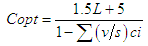 | (19) |
Where:Copt = Optimum cycle length (s);L = Sum of the lost time from all phases (s);(v/s)ci = Flow ratio, which is the design flow rate of critical lane group divided by saturation flow rate [11].However, to demonstrate the calculation of Webster’s optimal cycle length, total lost time (L) needs to be assumed since the method is delay-based. According to HCM, the sum of the startup and clearance delays are defined as a default value of 4 seconds per phase; thus, the total lost time for a four-phase signal control is estimated as 16 seconds per cycle [7]. Next, critical movements, critical flow of each phase, saturation flow rate, and number of lanes were investigated to calculate the delay-based optimal cycle length based on Webster’s method. In addition, MNS, MNL, KWS, and KEL are found to be the critical movements of phase T1, T2, T3, and T4, respectively. Although saturation flow rates are found to differ from region to region, due to the aggressiveness of the local drivers [3], HCM recommends that approaches with lower approach speeds of less than 31 mph (50 km/h) normally have saturation flow rate of 1,800 vehicles per lane per hour [4]. As a result, the arrival rates, as shown in Table 7, were converted to vehicles per hour (vph) unit in order to perform the calculation. Equation 19 was then applied with these parameters, and the Webster’s optimal cycle length turned out to be 66 seconds, as illustrated in Table 6. The calculation shows that the delay-based optimal cycle length is extremely close to the suggested 67-second cycle length performed on the basis of queue length optimization via linear programming. However, the optimal cycle length obtained from Webster’s method lacks of inclusion of pedestrian and vehicle queue length constraints, while the startup and clearance delays were excluded from the queue-length based linear programming method (L=0), according to the assumptions set in this study.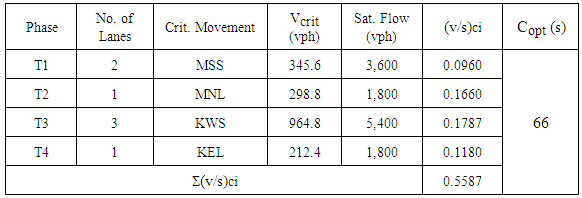 | Table 6. Webster’s delay-based optimal cycle length calculation |
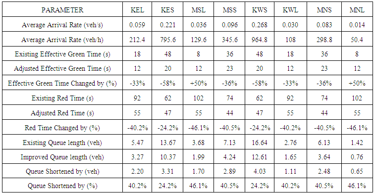 | Table 7. Parameters of the existing and suggested signal control systems of each movement |
6. Discussion and Conclusions
The existing effective green times, as shown in Table 7, indicate that the existing signal control opts to accommodate the through movement flows on both Kapiolani Boulevard and McCully Street by assigning the relatively longer effective green times, compared with the green times for left turns, in one cycle. To specify, the existing effective green time for Kapiolani through movements is 48 seconds, while 18-second effective green time is allowed for the left turns. Besides, the similar manner is adopted for effective green times on McCully turns. The decision may be made based on the relatively higher arrival rates on the through lanes, compared with the arrival rates on the left-turn lanes. However, effective green times for most of the turns in the existing system themselves are relatively longer than those effective green times suggested by the optimal solution. The phases and sequencing of both signal controls can be illustrated via a diagram, as presented in Figure 7. When the impact of the adjusted effective green times on vehicle queue lengths is considered, it is found that the queue lengths of all the movements are shortened by various amounts when the optimal solution is adopted, as shown in Figure 8. However, the vehicle queue lengths of each pair of movements, which are governed by the same green time, reduce by the same percentage. To illustrate, on McCully Street, the queue lengths of the through movements reduce by 40.5%, while the queue lengths of the left turns reduce by 46.1%. Likewise, on Kapiolani Boulevard, the queue lengths of the through movements reduce by 24.2%, while the queue lengths of the left turns reduce by 40.2%, as shown in Table 7. Obviously, such results occur since each pair of movements are governed by the same red time. Furthermore, ones can notice that the average vehicle arrival rates of Kapiolani through movements are the two highest arrival rates, 0.26833 veh/s (965 vph) and 0.22056 veh/s (796 vph), respectively, for westbound and eastbound. In addition, the existing effective green times for Kapiolani through movements are relatively longer than the effective green times suggested by the optimal solution. 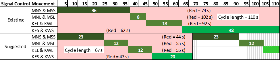 | Figure 7. The diagram presents phases and cycle lengths of the existing and the suggested pretimed signal controls |
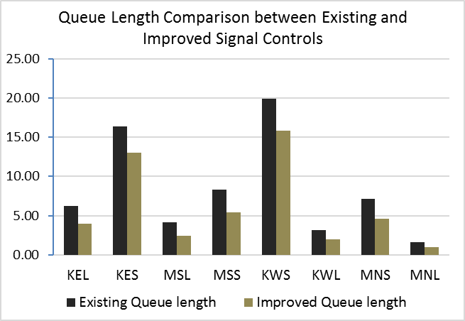 | Figure 8. Comparison between vehicle queue lengths of the existing and suggested signal control systems |
However, the vehicle queue lengths of both the Kapiolani through movements decline even though their effective green time, T3, is suggested to reduce from 48 seconds to 20 seconds, which is a 58.3% reduction. Therefore, the finding suggests that the number of idle vehicles on a specific movement does not solely depend on its green time. On the other hand, the red time for these movements are suggested to reduce from 62 seconds to 47 seconds, which is reduced by exactly 24.2% as same as the reduction in queue length. When the red time of each pair of movements is shortened, fewer vehicles consolidate on those lanes during the period. In other words, the longer green time assignment on the movements that possess relatively higher vehicle arrival rates does not necessarily mean that the number of vehicles queuing at an intersection, as a whole, is reduced by as much as the shorter red time on those movements. This can happen because the longer green phases may create an excessively long cycle length that generates longer queues on the perpendicular movements as well.Furthermore, let’s consider a case when only Kapiolani and McCully through movements are exclusively scoped, while left turns are restricted, in order to highlight the direct impact of effective red time on each movement’s queue length. In this case, green time for the McCully through movements will directly be red time for the Kapiolani through movements, and vice versa. The existing system adopts a 36-second duration as an effective green time for McCully through movements, which also means that the red time for the Kapiolani through movement is directly 36 seconds. Since the aggregate vehicle arrival rate on Kapiolani through movements is 0.489 veh/s (1,760 vph), the total number of vehicles expected to queue on Kapiolani Boulevard in one loop is 17.6 vehicles. However, for the same aggregate vehicle arrival rate on Kapiolani through movements under the red time of 23 seconds, as assigned by LINDO, the total number of vehicles expected to queue on Kapiolani in one loop is only 11.2 vehicles, which means the overall queue length on Kapiolani is shortened by 6.4 vehicles. It also means that the first vehicle in the line under the existing system may need to wait up to 36 seconds on Kapiolani until the traffic signal turns to green, while the same vehicle may take up to only 23 seconds waiting for green indication when the suggested system is adopted.Moreover, the queue-length based optimal cycle length of 67 seconds suggested by this study is only one second different from the 66-second optimal cycle length based on Webster’s delay-based approach. Although different inputs and assumptions were applied, such similar results obtained from both methods validate the potential of this cycle length on both queue and delay optimizations. Consequently, it can be inferred from the study that the existing 110-second cycle adopted by the Kapiolani-McCully intersection is too long; therefore, it encourages an excessive number of vehicles to be jammed there during the long red time of each movement. In other words, the suggested model improves the traffic flow at the intersection due to the shorter 67-second cycle, and the shorter red time for each movement. Although the number of vehicles queuing at the intersection during a cycle can be reduced in greater degree if the red time of each movement is shortened, the solution is restricted by such constraints as crosswalk safety and vehicle flow constraints.
7. Nomenclature
The following symbols are used in this paper:KWL = Average vehicle arrival rate of the west Kapiolani left-turn lane;KWS = Average vehicle arrival rate of the west Kapiolani through lanes;MNS = Average vehicle arrival rate of the north McCully through lanes;MNL = Average vehicle arrival rate of the north McCully left-turn lane;KEL = Average vehicle arrival rate of the east Kapiolani left-turn lane;KES = Average vehicle arrival rate of the east Kapiolani through lanes;MSS = Average vehicle arrival rate of the south McCully through lanes;MSL = Average vehicle arrival rate of the south McCully left-turn lane;T1 = Effective green time for the MNS and MSS phases;T2 = Effective green time for the MNL and MSL phases;T3 = Effective green time for the KWS and KES phases; T4 = Effective green time for the KWL and KEL phases.
ACKNOWLEDGEMENTS
The authors wish to thank Manuela Melo for help in formatting the article.
References
| [1] | City and County of Honolulu, Chapter 15: Traffic Code Article, Sec. 15-7.2, Revised Ordinances of Honolulu 1990. Retrieved from https://www.honolulu.gov/rep/site/ocs/roh/ROH_Chapter_15a1_9_.pdf, accessed April, 2017. |
| [2] | FHWA, Manual on Uniform Traffic Control Devices, Chapter 4E. Pedestrian Control Features, Sec. 4E.06 Pedestrian Intervals and Signal Phases, 2009. Retrieved from https://mutcd.fhwa.dot.gov/htm/2009r1r2/part4/part4e.htm, accessed Nov, 2016. |
| [3] | Hamad, K., and Abuhamda, H., "Estimating base saturation flow rate for selected signalized intersections in Doha, Qatar." Journal of Traffic and Logistics Engineering Vol 3.2, 2015, pp. 168-171. |
| [4] | Highway Capacity Manual, Transportation Research Board of the National Academies, Washington D.C., 2010. |
| [5] | Humphrey, M., Dona, S., Singh, A., Swe, T.T., “A Comparison of Traffic Performance in Highly Congested Urban Areas,” International Journal of Traffic and Transportation Engineering, Vol. 5 (5), pp. 47-63, 2016. |
| [6] | Jacobs, A.J., “The New Domestic Automakers in the United States and Canada: History, Impacts, and Prospects,” Lexington Books, Lanham, Maryland, 2015. |
| [7] | Koonce, P., et al. Traffic signal timing manual. No. FHWA-HOP-08-024. 2008, pp. 3-7. |
| [8] | Li, X., G. Li, S. Pang, X. Yang, and J. Tian. Signal timing of intersections using integrated optimization of traffic quality, emissions and fuel consumption: a note. Transportation Research Part D: Transport and Environment, Vol. 9 (5), pp. 401–407, 2004. |
| [9] | Longley, D., "A Control Strategy for Congested Computer Controlled Traffic Network", Transportation Research. Vol. 2, 1968, pp 391-408. |
| [10] | Ma., “Multi-criteria evaluation of optimal signal strategies using traffic simulation and evolutionary algorithms,” 6th International Congress on Environmental Modelling and Software, Leipzig, Germany, pp. 120-127, 2012. |
| [11] | Mannering, F., and Washburn, S., Principles of Highway Engineering and Traffic Analysis, 6th Edition, John Wiley & Sons, Inc., Hoboken, NJ, 2016. |
| [12] | Stevanovic, A., J. Stevanovic, K. Zhang, and S. Batterman. “Optimizing traffic control to reduce fuel consumption and vehicular emissions,” Transportation Research Record: Journal of the Transportation Research Board, No. 2128, Transportation Research Board of the National Academies, Washington, D.C., 2009, pp. 105–113. |
| [13] | Winston, W., Operations Research: Applications and Algorithms, 4th Edition, Thomson Brooks/Cole Publishing, Belmont, CA, 2004. |
| [14] | Zakariya, A. Y., and Rabia, S. I., Estimating the minimum delay optimal cycle length based on a time-dependent delay formula. Alexandria Engineering Journal, 55(3), 2016, pp. 2509-2514. |
| [15] | Zhang, L., Yin, Y. and Lou, Y., “Robust signal timing for arterials under day-to-day demand variations,” Transportation Research Record: Journal of the Transportation Research Board, No. 2192, Transportation Research Board of the National Academies, Washington, D.C., 2010, pp. 156–166. |

 Abstract
 Reference
 Full-Text PDF
 Full-text HTML