Mehrnaz Doustmohammadi1, Michael Anderson1, Sumalatha Kesaveraddy1, Steven Jones2
1Department of Civil and Environmental Engineering, University of Alabama in Huntsville, Huntsville, USA
2Department of Civil, Construction and Environmental Engineering, University of Alabama, Tuscaloosa, USA
Correspondence to: Mehrnaz Doustmohammadi, Department of Civil and Environmental Engineering, University of Alabama in Huntsville, Huntsville, USA.
| Email: |  |
Copyright © 2017 Scientific & Academic Publishing. All Rights Reserved.
This work is licensed under the Creative Commons Attribution International License (CC BY).
http://creativecommons.org/licenses/by/4.0/

Abstract
Travel demand models are used to forecast future traffic roadway traffic volumes to identify congestion and assist in the allocation of resources for transportation infrastructure and capacity improvements. The accuracy of these models is evaluated in this work through the examination of five travel demand models developed in the 1990s forecasting 2015 traffic. The focus of this effort differs from previous studies through the evaluation of the accuracy of the forecasted number of trips and also includes the accuracy of the assigned volumes to current travel demand model counts for the city that had the best trip results. A series of statistical analysis were performed to determine the level of accuracy of the forecasts. The results of the study demonstrate the home-based-work production values and home-based-other production values had the highest accuracy while home-based-other attraction values had the lowest accuracy.
Keywords:
Model Accuracy, Travel Demand Models, Statistical Analysis
Cite this paper: Mehrnaz Doustmohammadi, Michael Anderson, Sumalatha Kesaveraddy, Steven Jones, Examining Model Accuracy: How Well did We do in the 1990’s Predicting 2015, International Journal of Traffic and Transportation Engineering, Vol. 6 No. 1, 2017, pp. 15-21. doi: 10.5923/j.ijtte.20170601.03.
1. Introduction
Travel demand models are used to determine the best roadways to improve to ensure smooth traffic flow through the allocation of resources for capacity improvement projects. The modeling process in smaller urban communities tends to follow the conventional, four step sequential process: trip generation, trip distribution, mode choice, and traffic assignment (however, in smaller urban communities the mode choice step is often not included as transit represents a very minor percent of total trips). These travel models are updated every few years, as required by transportation legislation, therefore, it is rare that an analysis of the accuracy of the model is assessed. While it is common to focus on individual studies to improve specific components within the models, it is rare that the holistic view of accuracy of the entire modeling process is conducted. Previous studies have been conducted to assess the accuracy of travel models [1-3]; in these studies, the comparison of traffic counts forecasted and the actual traffic were compared through a variety of statistical methods. This study used travel demand model data from five communities in Alabama: Anniston, Auburn-Opelika, Gadsden, Huntsville and Tuscaloosa. The analysis focused on the number of trip generated and traffic volumes for different levels for different communities. Within each community, a selection of zones was used for the study that best supported the effort, as explained in the paper.This study examines the accuracy of forecast made in the in the 1990s to forecast current socio-economic data. The analysis is made through the examination of trips generated, by purpose, at both the aggregate level and the zonal level. This analysis was performed for five individual communities in Alabama where a model was available that was developed in the 1990s and a model was available with the current base year validated to existing socio-economic data and traffic counts. In addition, a comparison was performed for one community with the best forecast accuracy to compare traffic counts that were forecasted and actual traffic counts during the forecast year. The paper concludes that households are generally stable for forecasting while retail employment has a large influence on making wrong decisions.
2. Data
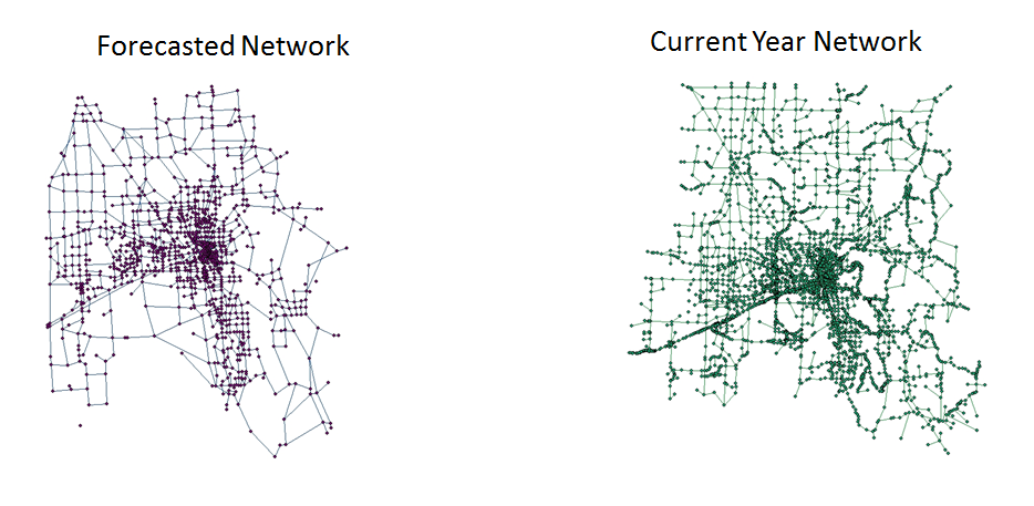
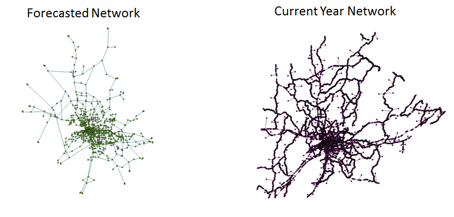
The data collected for the study include the travel demand network files, node and link data, along with trips generated by purpose for both the original forecast performed almost 20-25 year prior and the current files. The data used in the study were all based on TRANPLAN from the original forecast and VOYAGER for the current models. The cities used in the study were all from Alabama and include: Anniston, Auburn-Opelika, Gadsden, Huntsville and Tuscaloosa. The travel networks are shown in Figures 1-5 for the different communities. As can be seen from the figures, the urban boundaries for the communities were changed as a result of changes in rules and population growth between the 1990 Census and the 2010 Census, the years in which the different models and urban boundaries would have been based upon. The trips generated use three standard purposes: home-based work (HBW), Home-based other (HBO) and non-home-based (NHB). Within Alabama, the production values for individual zones are based on a series of cross-classification tables and the attractions are based on regression equations. For the trip productions, first the zonal income determines the number of vehicles owned, second the trips per household by vehicles owned determine trips per household and finally the trips are divided into purpose. For the trip attractions, regression equations have been developed and are based on employment, both retail and non-retail, and households and school enrollment. The data collected were maintained, manipulated and evaluated using ArcGIS and Excel.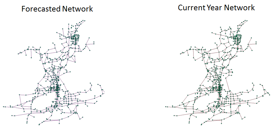 | Figure 1. Anniston Network Comparison |
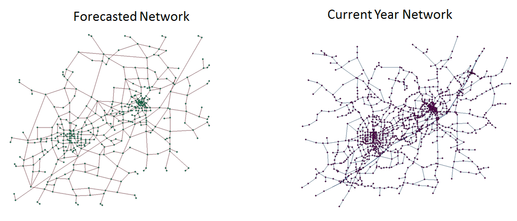 | Figure 2. Auburn-Opelika Network Comparison |
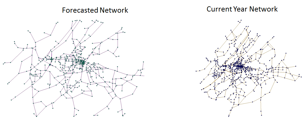 | Figure 3. Gadsden Network Comparison |
 | Figure 4. Huntsville Network Comparison |
 | Figure 5. Tuscaloosa Network Comparison |
3. Methodology
The analysis of the model accuracy was performed at three levels. The highest level was to determine the aggregate number of trips forecasted and actual, by purpose (HBW, HBO and NHB). The second level was to determine the difference in the forecast for individual zones and the actual number of trips for individual zones for each of the three trip purposes. The third level was to examine the actual traffic volume forecasted and actual traffic volumes on roadways. The first two analysis were performed for all five communities in the study, with modifications, and the third analyze was performed for Anniston only.For the first analysis, care was taken to ensure that the aggregate number of trips by purpose was reasonable. Due to the expansion of urban boundaries over the time period, care was taken to ensure that additional zones added to the current year models were not included in the comparison. The process involved using ArcGIS to display both models and only select the zones from the current year model that reflected the extent of the urban boundary from the original forecast. The reasoning behind this was that the growth in the community occurred on the outskirts of the community as urban sprawl incorporated previous rural land for subdivisions and commercial establishments. The analysis only used zones that were present in the previous model and current model. As such, there were several zones from the current year model not included in the aggregate totals.For the second analysis, care was taken to ensure that the individual zone trip values by purpose were comparable. Due to the changes in traffic analysis zone boundaries, splitting of zones and other modification, only zones where the boundaries were consistent between the current year model and the original forecast were used in the analysis. The process that was used involved developing Thiessen Polygons developed for both the current year model and original forecast and seeking locations where there was significant overlap between the layers. The locations where the overlap was significant and there was a one-to-one correspondence between layers were used in the analysis.For the final analysis, the roadways from the selected community that were obvious in both the current year model and the original forecast were selected and used in the analysis.
4. Case Study and Results
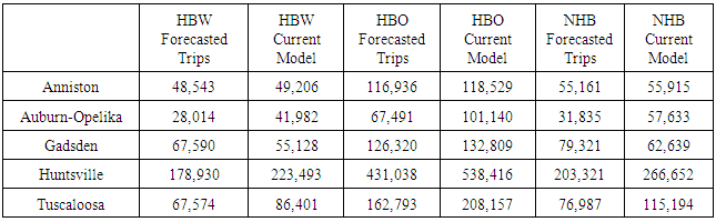
The case study and results were collected for the different communities using the different analysis previously discussed.The aggregate analysis examining the number of trips and the percent difference by the different trip purposes for the communities is shown in Table 1 and Table 2. As can be seen in the table, all communities except Gadsden for HBW and NHB, the forecast was less than the actual number of trips. The aggregate number of trips was closest for Anniston and the forecast for Auburn-Opelika was the largest difference. While this is definitely not definitive of the entire community, as the urban boundary changed between the forecast and current year model, this shows that the aggregate socio-economic data tended to under-predict the actual amount of trips expected in the communities.Table 1. Total Trips by Purpose for the Cities
 |
| |
|
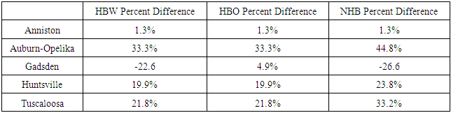
Table 2. Percent Difference in Trips by Purpose for the Cities
 |
| |
|
The second analysis was to examine individual zones from the communities where the boundaries were consistent between the two models. The analysis performed included several statistical tests to assess the accuracy of the original forecast to match the current year model. The statistical analysis performed included a Mann-Whitney U Test, GEH statistics, percent root mean square error and the Nash-Sutcliffe statistic. The Mann-Whitley U Test is non-parametric test used to compare if two independent samples have the same median [4]. To perform the test, certain assumptions must be met including: random populations, independence within the samples, and an ordinal measurement scale is assumed [4]. To ensure the appropriateness of the Mann-Whitney U Test, the variance from the forecasted model and the current year model must be the same [4]. This is performed through the use of Bonett’s Two Variable Method, which is used to determine if the variances are the same [5]. After determining the appropriateness of the variance, the Mann-Whitney U Test is performed using Equation 1.Equation 1:  Where: U = Mann-Whitney U Test statisticn1 = Smaple Sizen2 = Sample Size 2Ri = Rank of the sample sizeThe interpretation of the Mann-Whitney U Test results is based on the P-Value. If the P-Value is less than 0.05, then the data have the different medians and can be considered not the same. If the P-Value is greater than 0.05, then it doesn’t ensure that the data are similar, and other tests are added to provide more detail. A GEH statistic was calculated using Equation 2 [3]. Numerically, a small GEH value if considered a good fit while a value of zero is obtained when the forecast and actual value are the same [3]. For analysis purposes, a value of less than 5 is considered good, between 5 and 10 is considered decent, and greater than 10 is not considered to be is quality [6].Equation 2:
  Where:GEH = Test statisticM = Model valueC = Count valuePercent Root Mean Square Error was calculated as a metric using equation 3 [7]. Percent Root Mean Square Error values for validation of travel models generally less than 40 represent reasonable values for traffic counts for base year conditions [7]. Given the nature of the forecast and the use of trip data, values less than 100 were taken to be reasonable for this study.Equation 3:
  Where:RMSE = Test statisticx1 = value from model 1x2 = value from model 2n = sample sizeNash-Sutcliffe was calculated as a metric using equation 4 [8]. Numerically, the value of the N-S coefficient ranges from 1 to –infinity where a value of 1 indicates that the forecast and actual value are the same, a value of zero indicates that the average value of all the current year data is as good as the forecast methodology and a negative value indicates that the forecast is worse than taking the average of the values and using them [8].Equation 4:
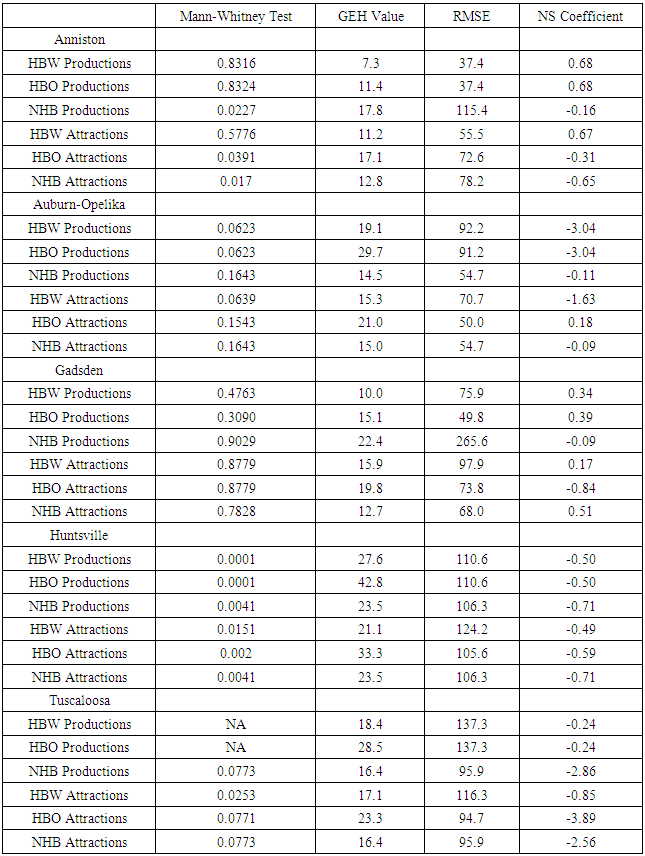
  Where:E = Test StatisticQo = model value 1Qm = model value 2(Qo) ̅= mean of model 1The values for the different analysis are shown in Table 3. Note that if the Mann-Whitney U Test is not applicable, then no value is entered in the table 3.
Table 3. Statistical Results for Individual Zone Analysis
 |
| |
|
As can be seen from Table 3, while not ideal, the HBW productions and HBO productions tended to perform slightly better for most cities. This result is expected because this trip purpose is based on households in the community and not likely to change greatly during the forecast, especially in the area where the households were already somewhat established. Essentially, the number of households in the zone is expected to remain constant for zones with complete buildout of the available land or increase slightly in locations where there is expected to be some moderate growth. Surprisingly, in none of the zones for HBW and HBO were the trips the same, indicating that the number of households had reached a maximum for the zone and there was no room for growth. Also from Table 3, HBO attractions tended to be the worse from the forecast. This result is also not a complete surprise as this trip purpose is heavily dependent on retail employment in the zone. The ability to forecast retail employment accurately 20-25 year into the future is a very difficult task indeed.The third analysis was performed examining the specific roadway volume comparison. For this test, only the data for Anniston were used as this community had the best results from the aggregate and zonal comparison. ArcGIS was used to select roadways that had the exact geometry from the forecast model and current year model, only these roadways were included in the analysis. A scatter plot of the forecasted data from the 1990s and the current base year model volume is shown in Figure 6.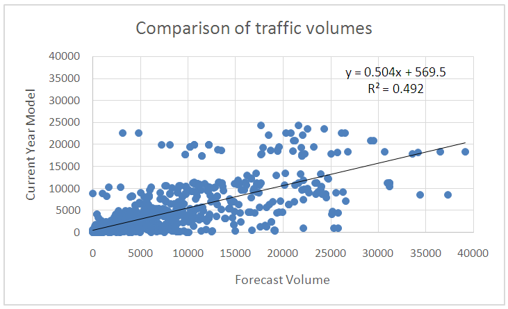 | Figure 6. Comparisons of Traffic Volumes in Anniston |
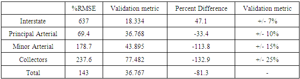
The statistical analysis performed for the traffic volume comparison included the calculation of the GEH statistic, percent root mean square error (%RMSE) and percent difference. The average GEH statistic for the data was determined to be 49.9. This value is not ideal and shows the influence or effects in the modeling process associated with the differences in zonal values and how those errors are compounded through trip distribution and traffic assignment. The use of %RMSE and percent difference calculated for different roadway functional classification and these measures were selected to associate the results with target validation results for developing a base year travel demand model, see Table 4 [8]. As with the zonal data, the expectation of achieving base year validation level results is unreasonable, but the values are included as a reference of quality.Table 4. Traffic Count Statistics
 |
| |
|
A further examination of the roadways based on the difference between zones looked specifically at the Home Based Other Attractions (HBWa). There were three zones in the model where the difference in HBWa was greater than 7,000 trips in the current year model versus the forecast model, see Figure 7 for the location. The extreme difference in the number of trips attracted to this general area in Anniston due to a lack of retail employment, will lead to a significant difference in traffic counts between the models. However, changes in retail are difficult to predict, especially in the 20-25 year time frame, as retail employment and locations are very short-term.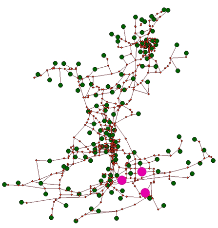 | Figure 7. Location of Extremely High HBWa Values |
5. Conclusions
This paper examined the accuracy of travel demand models developed in the 1990’s and their ability to forecast trips and traffic volumes in 2015. The aggregate number of trips for the models was almost always underestimated compared to the development that actually occurred. When examining zonal values, home based work and home based other production values tended to be closer to actual value. This is theorized to be based on the notion that these two trip purposes are based on the number of households in the community, which is often a forecasted value that is an increase of the number of households that are in the base year – often households are not removed - and in zone with complete growth – there is not ample land to build new households. The inability to accurately forecast retail employment, the leading variable in home based other attraction values, lead to larger difference in this purposes.Finally, the location of retail employment has a large influence on the traffic count forecasted from the model and can lead to significant differences in volumes. Unfortunately, retail employment is difficult to forecast more than a few years into the future as companies are often adding retail employment and moving retail employment to larger stores on new parcels.Overall, the ability of the model to forecast trips and traffic is beneficial and leads to the support to update the models at a regular interval to ensure the models are using the current base year conditions to improve the ability to forecast.
References
| [1] | Anderson, Michael D., Walter C. Vodrazka Jr, and Rreginald R. Souleyrette. "Iowa Travel Model Performance, Twenty Years Later." Transportation, Land Use and Air Quality Conference. (1998). |
| [2] | Parthasarathi, Pavithra and David Levinson. "Post-Construction Evaluation of Traffic Forecast Accuracy." Transport Policy 17.6 (2010): 428-443. |
| [3] | Buck, Karl and Mike Sillence. "A Review of the Accuracy of Wisconsin’s Traffic Forecasting Tools." Transportation Research Board 93rd Annual Meeting. No. 14-1717. 2014. |
| [4] | Http://www.statisticssolutions.com/mann-whitney-u-test. Accessed july 19, 2016. |
| [5] | Http://support.minitab.com/en-us/minitab/17/bonetts_method_two_variances.pdf. Accessed july 19, 2016. |
| [6] | Horowitz, Alan et al. Analytical Travel Forecasting Approaches for Project-Level Planning and Design. No. Project 08-83. 2014. |
| [7] | Cambridge Systematics. "Travel Model Validation and Reasonableness Checking Manual." Travel Model Improvement Program. (2010). |
| [8] | Nash, Eamonn and Jonh Sutcliffe. "River Flow Forecasting through Conceptual Models Part i—A Discussion of Principles." Journal of Hydrology 10.3 (1970): 282-290. |

 Abstract
 Reference
 Full-Text PDF
 Full-text HTML