1. Introduction

Traffic assignment is a key components of transportation models, which relates travel demand to infrastructure supply. Traffic assignment models are widely used as a tool to assist in making decisions in mobility and infrastructure transportation planning. These tools can help in analyzing congestion issues, and can predict the consequences of certain measurements, like adding an extra lane, building a new road, raising the maximum allowed speed or applying road pricing. For the few past decades, the traditional trip-based approach to transportation modeling has dominated the planning process. The trip-based method includes: trip generation, trip distribution, modal split and trip assignment. The first three steps of the trip-based method typically constitute the transportation demand side, while trip assignment normally represents the transportation supply side.

Traffic assignment models are available in numerous formulations. From a basic all-or-nothing formulation, which assigns all traffic between Origin-Destination pairs to the shortest path, to static models, to more complicated dynamic models. On the supply side, conventional techniques of trip assignment based on static traffic assignment (STA) have been employed for decades. Traffic assignment models can be either static or dynamic. Within dynamic models, the traffic demand (OD-matrix) can change through time, while within a static model it is assumed that the traffic demand is constant through time. The limitations of the static assignment procedures and the increase in software’s and computing capacity have allowed this field to move toward more behaviorally realistic dynamic traffic assignment (DTA) models.

(DTA) models are becoming increasingly popular among researchers. Dynamic methods were first developed by Merchant and Nemhauser (M – N Model), and in the past two decades, dynamic models have been extensively researched and developed into complex mathematical formulations of route choices. DTA models are used for estimating and predicting time-varying traffic conditions in road networks. Meanwhile, static traffic assignment (STA) models are criticized for inadequate representation of the utility maximization aspect and for being unable to handle situations where the travel demand exceeds road capacity or where congestion is not continuous. DTA techniques offer a number of advantages relative to the STA methods including; capturing time-dependent interactions of the travel demand and supply of the network; capability to capture traffic congestion build-up and dissipation; accommodating the effect of ramp-meters and traffic lights on the network; modeling the effects of ITS technologies; and representing the network at a disaggregate level [1].

This paper handles the findings of three recent dynamic traffic assignment models, namely; 1) A dynamic traffic assignment model for highly congested urban networks; 2) System-optimal dynamic traffic assignment with and without queue spillback: Its path-based formulation and solution via approximate path marginal cost; and 3) A dynamic traffic assignment model for the assessment of moving bottlenecks. The first model offers a method to address the challenges of dealing with highly congested urban networks that poses long queues, short links, and a lot of closely spaced ramps, the second model offers a method to minimize the total path marginal cost of a network based on two queuing models, and the third model offers a method to assess the effect of bottlenecks on the network performance.

2. Literature Review

Traffic assignment models constitute an integral part of the travel demand modeling framework, and it has long been recognized as the last step of the traditional four step travel demand modeling process and widely used as an evaluation tool for a variety of urban, rural, and regional traffic network analyses. The basic principles behind the deterministic static models were defined by Wardrop, which were further refined by Frank and Wolfe and LeBlanc [2]. As the modeling procedures further developed, probabilistic models of route choice were also presented, but were not considered suitable for large congested networks [3]. A set of nonlinear programming modeling was introduced by Beckmann for the deterministic traffic assignment models with the first and second Wardropian principles, and various types of traffic assignment models have been developed in the past two decades. The developed models have been produced as optimization programs, variational inequalities, complementarity systems, or fixed-point problems. The two Wardrop’s principles have also been used to produce stochastic models by optimization programs, including the stochastic user-equilibrium (SUE) model and the stochastic system-optimal (SSO) model [4]. Dynamic traffic assignment (DTA) has been a topic of substantial research during the past two decades, and they are gradually maturing, and their actual use is expanded to transportation planning studies. The main characteristic of DTA models is that they are able to capture the spatio-temporal trajectory of each individual vehicle, starting from the origin up to the destination. DTA models are usually utilized as replacement of the classic static traffic assignment (STA) models, for various applications. STA models are not able to capture the dynamics of traffic flow, since they are using link travel cost functions which depend only on the traffic flow on this link, without taking into account the effects on the traffic flow of other links. In a static model, inflow to a link is always equal to the outflow, and the travel time increases as the inflow and outflow (volume) increases. In dynamic models, if link outflow is lower than link inflow, link density will increase (congestion), and speed will decrease, and therefore link travel time will increase. Static models enforce the link FIFO rule (first-in, first-out), which means that all vehicles traveling on the link experience the same travel time. Most Dynamic models that move individual vehicles on discrete lanes of the roadway can model non-FIFO conditions, and thus effectively dealing with the queues and spillbacks [5].

DTA models can be classified into two categories: the first rely on analytical formulations, such as methods of mathematical programming, variational inequalities and optimal control theory and the second rely on simulation models [6]. Within those two broad categories, several types of DTA models exist.

Simulation-based DTA models deal with the flow of traffic and the spatial and temporal interactions, instead of a mathematical method. Simulation provides the convenient tool for modelling complex and congested dynamic traffic assignments, thus avoiding the difficulties associated with the use of mathematical methods. These models use traffic simulators for simulating traffic conditions, especially in networks where signal control exists and where a mathematical method is difficult to be used [7].

3. Discussion of Findings

1^st Model: A dynamic traffic assignment model for highly congested urban networks

This model offers an equilibrium dynamic traffic assignment (DTA) to address the challenges of dealing with highly congested urban networks that poses the following characteristics:

1. Thousands of directed links

2. A large number of existing short links

3. Frequent On-and-Off Ramps that are very closely spaced

4. Long Queues and Spillbacks throughout the network

5. High interferences from non-motorized traffic (bikes, pedestrians) at intersections

The model chose a study area located in Beijing, China and used a DynaMIT-P (Dynamic network assignment for the Management of Information to Travelers) simulation-based DTA system which has a built-in microscopic demand simulator that disaggregates the Origin-Destination (OD) flows and a mesoscopic supply simulator, which simulates the moving of vehicles with speeds governed by macroscopic speed-density relationships. Discrete choice framework was used to model the traveler’s decisions; the OD flows were converted into individual vehicles by the demand simulator. The chosen routes of the individual vehicles were then simulated in the mesoscopic supply simulator to obtain the network performance measurements such as time-dependent flows, travel times, and queue lengths [8].

The study area network consisted of 1698 nodes connected by 3180 directed links in an 18 square miles area. The dataset used included static demand during the AM peak hours for 2927 non-zero OD pairs, derived from the most recent household surveys and calibrated against counts and speeds from Remote Traffic Microwave Sensors (RTMSs) and travel times from Floating Car Data (FCD) with an initial time-dependent demand in 15 min intervals. The simulation ran from 6:00 am to 10:00 am, and approximately 630,000 vehicles were simulated. A total of 154 RTMSs detectors were deployed on the network, and it was reported that 140 of those sensors were functioning normally, providing a continuous 24-h traffic flow information. The count and travel time data were processed by Beijing Transportation Research Center (BTRC) in China, and the simulation was conducted in the Massachusetts Institute of Technology in Boston [8].

The optimization problem was solved using the Simultaneous Perturbation Stochastic Approximation (SPSA) algorithm, and in each SPSA iteration, DynaMIT-P was run three times, two of them to generate the gradient approximation, and a third run to produce traffic conditions with the adjusted parameters. The output link travel times from the 3^rd run were then used as input link travel times to the demand simulator of DynaMIT-P for the next SPSA iteration.

The Root mean square error (RMSE), and the Normalized root mean square error (RMSN) were used to measure the discrepancies between observed (yi) and simulated quantities as shown below, where S is the dimension of the unknown vector:

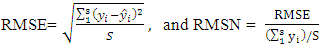There was an improvement in the objective function value at the end of calibration which indicated that the SPSA algorithm was appropriate for this particular problem. Throughout the simulation, queues appeared on 591 links, among which there were 33 spillbacks, and the longest spillback extends 3.20 km (1.99 miles) [8].

The model was used to capture the lane restrictions through using a lane group queuing approach that grouped the lanes according to their specific turning movements at intersections, and taking into account geometry changes, lane restrictions, and lane connections following the guideline given by Highway Capacity Manual (HCM). The lane group approach proved to be necessary in Beijing case study network, so that with a queuing part based on lane groups, the formed queues due to the limited capacity from another lane group were removed, and a large number of bottlenecks disappeared.

The model was also used to address the excessive congestion originated from the short links (which were usually around the length of a car). It was noticed that the congestion resulted from the short links were due to the vehicles that were moving very slowly on short links, and vehicles that were queuing unnecessarily upstream of a short link [8]. For a short segment, the density increases from zero whenever a car enters the segment. For instance, if the segment’s length equals to that of a typical car, then the density k could only be either 0 or k jam, which results in two possible calculated speed:

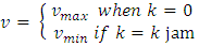If is lower than the average observed speed, this segment would always cause unrealistic congestion. The model used an increased starting value of the calibration variable of the minimum speed to the average observed speed for each of those short links, and restricted this value from deviating from the mean, and the method was effective for the Beijing study [8].

The model also addressed the acceptance capacity calculation for the short links. A queue for a given movement is formed on a lane group when either the output capacity of the lane group or the acceptance capacity of the downstream lane group is binding, and the actual flow rate of lane group j at time t can be found using the formula shown below [8]:

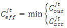where is the output capacity of lane group j at time t, and is the acceptance capacity of lane group j at time t. For short links, if the vehicle is moving, as soon as it moves out the lane group, another vehicle can be accepted, and hence, the acceptance capacity is not updated every time a vehicle is moved. The solution used in this model was to ignore the acceptance capacity constraint when there is no queue in the downstream segment by using the following formula:

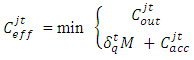where is a binary variable equals 1 if there is no queue on lane group j at time t and 0 otherwise, and M is an sufficiently large positive number. Using this formula, the excessive queuing phenomenon was eliminated in the case study.

The model also dealt with the impact of non-motorized traffic (bicycles and pedestrians) on vehicular traffic on road intersections by introducing the variable output capacity in the DTA model. The output capacity may not well reflect the traffic situation with significant interferences from bicycles and pedestrians, and the conflicts between bicycles/ pedestrians and vehicles are different during different times of the day because their flows are time-dependent, and accordingly the model assumed different values of the output capacity at different time-of-day to prevent causing capacity reductions for motorized traffic at the intersections, especially during rush hours [8].

The model was used to evaluate the benefit of the ‘Rotating No-Driving Day restriction’ scenario in Beijing, which was proposed by the Beijing municipal government to reduce pollution and relieve traffic by preventing private cars from being on the roads 1 weekday per week according to a rotation schedule based on license plate numbers. To model this scenario, the demand was decreased by 20%, and then compared with a control case that does not have the restriction, and it was found that the number of vehicles that reached their destination during the simulation time period was 8.4% less than the control (base) case, which indicated that adopting such a restriction policy on demand could significantly increase road efficiency and reduce congestion [8].

2^nd Model: System-optimal dynamic traffic assignment with and without queue spillback: Its path-based formulation and solution via approximate path marginal cost

This model offers a method of finding the path marginal cost (PMC), which represents the changes in network flow cost caused by one additional unit of flow on a path departed at a certain time. Path travel times/costs are obtained by dynamic network loading (DNL), and they depend on path flows which makes the evaluation of PMC very difficult in general networks [9].

This model adopted two widely used link models, the point queue (PQ) model, and the kinematic wave (LWR) (Lighthill and Whitham, 1955; Richards, 1956) model. Both address the dynamic congestion result from queuing, but differ in how to distribute the queues. The focus of this model was on how to calculate the PMC in general networks under PQ or LWR traffic dynamics.

The model used a link marginal cost (LMC) criteria to determine the path marginal cost (PMC) in four different cases namely; the single bottleneck queue; the sequential bottlenecks queues without merges and diverges; merged queues; and diverged queues [9].

In the single bottleneck case, and for a 3 links network, let’s say that the additional vehicle perturbation arrives on link 3 at time and the current queue disappears at time , and vehicles arriving at and depart at and , respectively. Then the arrival curve lifts up by one unit at time , and the vehicles arriving before are not affected by the perturbation, but only those vehicles arriving at time , where 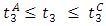are delayed by the perturbation, hence the LMC for link 3, and under both the PQ and the LWR models can be found as [9]:

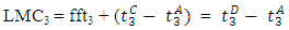, where fft₃ is the free flow travel time of link 3.

In the sequential bottlenecks without merges and diverges, the LMC for each of the links 1, 3, and under both the PQ and LWR models can be found as follows [9]:

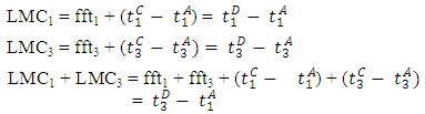In the case of the merged queues, and assuming that links 1 and 2 merge into link 3 where the flow perturbation passes through links 1 and 3, and under the PQ model, the vehicles at the head of the queue on link 2 can enter link 3, the cumulative curves on link 2 are not affected by the perturbation. If links 3 and 1 are not bottleneck links, then LMCs of both links are zero. If link 1 is a bottleneck link and link 3 is not, link 1 would be an isolated bottleneck link, and the single bottleneck case applies. If link 3 is a bottleneck link and link 1 is not, then the LMC of link 1 is zero. Under the LWR model, if link 3 is a bottleneck link, then queues form on both link 1 and link 2, and link 1 and link 2 look like PQ-modeled links with discharging rate of C₁ and C₂ that can be found as:

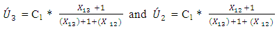
where, X_ij is the number of vehicles in the last cell of link i heading towards link j.

In case of the diverged queues, and assuming that links 1 diverges to link 2 and link 3 where the flow perturbation passes through links 1 and 3, and under the PQ model, the outflow of link 1 heading for link 3 and link 2, U₃ and U₂ respectively, may be affected by the perturbation when the bottleneck on link 1 is active as follows [9]:

with perturbation, and when link 2 is a bottleneck link, then:

And when link 2 is not a bottleneck, then:

The extra delay of any vehicle arriving on link 2 caused by the flow perturbation equals 1/C_1, and hence LMCs can be found as:

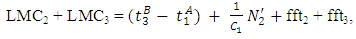where is the number of vehicles arriving on link 2 during and each of them is subject to an additional delay of 1/C₁ by the perturbation. Under the WLR model, the procedure is equivalent to the case of diverged queues under the PQ model where link 1 is a bottleneck and the cumulative curves of link 2 remains unchanged during arrival time .

Having the values of the LMCs in different cases as mentioned above facilitated determining of the path marginal cost PMC based on the time-dependent shortest path with respect to PMC by applying the decreasing order of time (DOT) algorithm. After that, the heuristic MSA algorithm was used to solve the formulation of the SO-DTA problem as follows [9]:

Step 1: Initialization, by selecting an initial flow pattern v = 0.

Step 2: Conducting a dynamic network loading based on (PQ or LWR models).

Step 3: Solving the least marginal cost for each O-D pairs

Step 4: Obtaining the auxiliary flow function through the assignment of all the demand onto the PMC

Step 5: calculating the formula

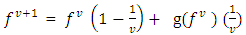Step 6: Terminating the iteration if convergence occurs, or going to Step 1 otherwise (9).

The approach used in this model to find the PMC from the LMC by analyzing the relationships between bottleneck links and computing the changes in cumulative flows on network links caused by an arbitrary flow perturbation is an innovative way to solve the SO-DTA problem on general networks.

3^rd Model: A dynamic traffic assignment model for the assessment of moving bottlenecks

Modeling the movements of individual vehicles in large urban networks is gradually becoming an achievable goal through the use of iterative assignment algorithms combined with traffic simulation models. The approach used in this model provides an overview on how to use the method of successive averages (MSA) as a methodology and an efficient event-based traffic simulation model for computing path travel times.

This model presents a dynamic traffic assignment (DTA) model that can evaluate the effects of moving bottlenecks on network performance in terms of travel times and traveling paths based on a mesoscopic simulation network-loading procedure by permitting traffic density and speed to vary along a link, and the simulation can capture the queue caused by the moving bottleneck. The following equation can be applied for the traffic flow that passes a moving bottleneck in a unit of time [10]

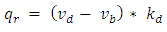where is the bottleneck speed; and are respectively the speed and density of the vehicles. Vehicles’ average speed in the moving queue can be calculated as

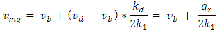where k₁ is the traffic density within the moving queue [10].

The mesoscopic simulation based algorithm used in this model utilized a bi-level segments, the upper and lower level, then the least marginal cost path with time dependent cost was determined, and the demand was loaded on the least marginal cost. The method of successive averages (MSA) was applied to obtain the set of splitting rates for each iteration, and the iterations were repeated until convergence was achieved [10].

The mesoscopic simulation used was based on a simulation of moving packets that follow macroscopic speed-density relationships, and the simulation terminated when all packets from all origins and departure-times had arrived at their desired destinations. The moving bottleneck within the simulation was integrated and the simulation accounted for variations in traffic density and speed along a given link. Each packet was considered as independent of others which indicated that the leading vehicle of the packet may travel at free-flow speed without being interrupted by following vehicles, and the distance k that the leading vehicle traveled in a period of time was the product of the link’s free-flow speed multiplied by the length of the period, and the density of the packet was calculated as the number of vehicles in the packet divided by k. The links that the bottleneck passed were divided into four segments: the bottleneck and the queue it induces (both of them denoted by the QMBa segment, in which the bottleneck was denoted by MB); two moving segments, one behind the moving bottleneck (denoted by M1a) and the second in front of it (denoted by M2a); and a queuing segment (Qa) at the end of the link. The queue-clearance rate (exit capacity) was the minimum of the available input capacity of downstream links, and the maximum number of vehicles that can pass through the head node intersection during one time interval [10].

The length of each of the four segments was continuously updated in simulation time intervals by the length of segment Q, the jam density, and the number of lanes. Then the location of the moving bottleneck was determined, and the length of M2, was calculated as the distance between the upstream end of segment Q and the front of segment QMB (the location of the moving bottleneck), and then the location of the end of segment QMB was determined, and the length of M1was the distance between this location and the tail node of the link [10].

The speed of the moving queue was found as follows:

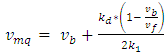, where k₁ is the traffic density within the moving queue

The rate at which vehicles passed the moving bottleneck was calculated using the formula:

Where is the location of the packet at time and is the packet length, and the location of the upstream end of the moving queue was calculated in each simulation time interval according to the bottleneck location and the number of vehicles in the packets located within the moving queue. Link travel times and marginal travel time in the model were measured directly in the simulation at the packet level. The model handled spillbacks by physical queues, which track the length of the queue with respect to the link’s length; exit capacities, which considered the available input capacity of downstream links and were reset to zero when spillback occurred; a changeable simulation time interval (STI), which was set to a minimum defined length when spillback occurred. Discharge rates were calculated for each link in each simulation time interval, based on the splitting-rate variables, and the exit capacity of each link was set to the minimum of two values: the maximum number of vehicles that can pass through the head node intersection within one time interval; and the input capacity of downstream links. The exit capacity of flow links at signalized intersections was based on the user’s supply saturation flow (s), effective green times (g), and cycle length (C), and on the left-turn (LT) factor, as follows [10]:

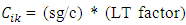, and the LT factor was approximated according to the number of lanes, the percentage of left-turns, and the volume/capacity ratio of opposing flows.

The simulation showed that the average trip time increases inversely with the moving bottleneck speed. That is, as the moving bottleneck travels faster, its disturbance to traffic is smaller, and therefore the average travel time in the network is lower, because as the bottleneck travels faster, its speed becomes closer to the average traffic speed, and therefore it creates less interruption to traffic, and the moving bottleneck affects the optimal distribution of trips on the available paths in the network attained by DSO, as it diverts traffic from links on which it is traveling to other links. The simulation also showed that the disruption of the moving bottleneck is a function of overall network congestion, and this continues until the network is loaded to a certain demand level or maximal point beyond which the moving bottleneck causes less delay to the traffic as average congestion grows [10].

4. Conclusions

Traffic assignment models are an important part of the trip modelling process. The output from these models is used in decision making process regarding transportation infrastructure investments. Many types of traffic assignment models are available from a basic all-or-nothing formulation, to static models, to more recent dynamic models. The limitations of the static assignment models (STA) and the increase in software’s and computing capacity have allowed researchers to move toward more realistic dynamic traffic assignment (DTA) models.

This paper provides a summary of the findings that were achieved by three recent dynamic traffic assignment models, the first one was: (A dynamic traffic assignment model for highly congested urban networks) that offers an equilibrium (DTA) to address the challenges of dealing with highly congested urban networks that poses thousands of directed links, a large number of existing short links, frequent On-and-Off ramps that are very closely spaced, long queues and spillbacks throughout the network, and high interferences from non-motorized traffic (bikes, pedestrians) at intersections. The model used a DynaMIT-P simulation-based DTA system to obtain the network performance measurements such as time-dependent flows, travel times, and queue lengths. The findings of the model were:

Ÿ Captured the lane restrictions through using a lane group queuing approach that grouped the lanes according to their specific turning movements, and the formed queues due to the limited capacity from another lane group were removed, and a large number of bottlenecks disappeared.

Ÿ Addressed the excessive congestion originated from the short links, and the abnormal queuing phenomenon was eliminated in the case study.

Ÿ Dealt with the impact of non-motorized traffic (bicycles and pedestrians) on vehicular traffic on road intersections by introducing the variable output capacity in the DTA model to prevent causing capacity reductions for motorized traffic, especially during rush hours.

Ÿ Evaluated the benefit of the ‘Rotating No-Driving Day restriction policy’ that could significantly increase road efficiency and reduce congestion.

Ÿ Presented a route choice model that can account for overlapping routes.

The second model was: (System-optimal dynamic traffic assignment with and without queue spillback: Its path-based formulation and solution via approximate path marginal cost) that offers a method of finding the path marginal cost (PMC), a central part of the path-based system-optimal dynamic traffic assignment (SO-DTA) problems through using a link marginal cost (LMC) criteria in four different cases namely; the single bottleneck queue; the sequential bottlenecks queues without merges and diverges; merged queues; and diverged queues. The findings of the model were:

Ÿ Adopted two frequently used link models, the point queue (PQ) model, and the kinematic wave (LWR) model to calculate the path marginal cost in general networks under the PQ and LWR traffic dynamics.

Ÿ Offered a new method of finding the path marginal cost for the System-Optimal dynamic traffic assignments through determining the link marginal cost procedure based on the time-dependent shortest path with respect to PMC by applying the decreasing order of time (DOT) algorithm.

The third model was: (A dynamic traffic assignment model for the assessment of moving bottlenecks), that presents a (DTA) model that evaluated the effects of moving bottlenecks on network performance in terms of travel times and traveling paths based on a mesoscopic simulation network-loading procedure. The findings of the model were:

Ÿ Showed that the average trip time increases inversely with the moving bottleneck speed.

Ÿ The moving bottleneck affected the optimal distribution of trips on the available paths in the network by diverting traffic from links on which it is traveling to other links.

Ÿ Showed that the disruption of the moving bottleneck is a function of overall network congestion, and this continues until the network is loaded to a maximal point beyond which the moving bottleneck causes less delay to the traffic as average congestion grows.