1. Introduction

Notwithstanding the development over the years, the vehicular traffic congestion is one of the most menacing challenges the word is facing. The congestion cost estimates were 1982 – $24 billion; 2000 – $94 billion; 2011 – $121 billion. Juan In spite of implementing some of the technologies, the cost of congestion is steadily rising; the estimated cost of congestion by the end of 2015 will be USD 133 billion. In spite of the developing technologies, its implementation, improved vehicle quality, driving sense and better infrastructure to name few catalytic parameters that can play an important role in mitigating vehicular traffic congestion, the congestion cost is increasing.

This means 1. The present technology has reduced the cost escalation but has not made significant inroads in containing traffic congestion 2. The prevailing technologies can only provide navigational assistance and inform about congestion but cannot stop congestion creation 3. The congestion information is not as real time because of inherent latency congestion detection 4. Lastly, congestion detection is not precise in terms of exact location of congestion due to the dynamic behavior of the traffic network.

The shortest distance path which is also shortest travel time path is the most preferred path and hence gets congested faster, creating the need for discovering alternate shortest travel distance path based since traffic congestion is a dynamic phenomenon. The technology driven solution continuously computes shortest paths based on travel time. The computation must reduce the latency which can be achieved by reducing the computation of alternate shortest travel path. This paper evaluates past research and proposes means to achieve efficient computation algorithmic boundary conditions.

2. Shortest Algorithms

Major contribution in Path Finding algorithm is made by algorithms like A*, BFS, Dijkstra's algorithm, HPA* and LPA* which are discussed below:

2.1. A*

Zarembo This algorithm uses heuristic function, to determine the order in which to traverse nodes. The heuristic F defined as:

F = G + H Cost to reach goal

G Exact cost of the path from initial node to the current node

H Admissible (not overestimated) cost of reaching the goal from current node

If H is overestimated the goal node is found faster but results are not necessarily optimal;

If H is underestimated, Best results but longer processing time

2.2. BFS

Breadth-first search (BFS) starts at the tree root and explores the neighbor nodes first, before moving to the next level neighbors. Zarembo BFS is a simple, traditional algorithm and the principles are used by Prim's minimal spanning tree algorithm and Dijkstra's single-source graph search algorithm. It neither takes advantage of available heuristics or reuse knowledge from previous search.

For a graph G = (V, E), BFS traverses edges of G from start node s to find nodes reachable from s. It calculates smallest number of edges from s to every reachable node and creates breadth-first-tree. The algorithm complexity in time obviously depends on O(│E│+│V│) when every edge and every nodes is visited. In reality O(│E│+│V│) can vary between O(│V│) and O(│V│²) depending on graph edge evaluation.

2.3. Dijkstra's Algorithm

Zarembo Biswas Dong The algorithm repeatedly selects nodes u ε V – S with the minimum shortest-path estimate, sums u and S, and relaxes all edges leaving u. Dijkstra's algorithm is "greedy" algorithm, it always chooses "the lightest" and "the nearest" node V – S to add to the set S. Dijkstra's algorithm holds set of nodes Q in linked list and finding node with minimal weight through linear search in set Q. The algorithm execution time is expressed as O(│E│+│V│²) and in worst case the performance is can be expressed as O(│E│+│V│Log│V│).

2.4. Hierarchical Path-Finding A*

Zarembo HPA* was developed by Adi Botea and his colleagues in 2004. It is about creating clusters and then finding shortest paths. A simple low resolution 2D grid s x s is created where s is the new grid. This is placed on the original graph and every node in the new grid is a cluster. Each cluster is a separate graph and an abstract graph is created to connect separate graphs. Border nodes consideration is important. If a node is on border and passable neighbor is in adjacent cluster, then it is considered connection between two graphs representing the clusters. If several adjacent connected nodes, then they are all combined into one entrance and connected in abstract graph. Internal edges in a cluster is obtained by running A* algorithm. HPA* is a 1% optimal path finding algorithm

2.5. Lifelong Planning A* (LPA*)

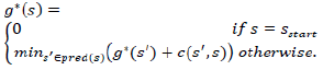
Zarembo LPA is ideally suited for problems where the graph keeps on changing either in terms of nodes or in terms of edge weights over a period of time. The functions used are as follows:

1) S is finite set of vertices of the graph

2) succ(s) denotes the set of successors of vertex s of S

3) pred(s) denotes the set of predecessors of vertex s of S

4) 0 < c (s, s’) ≤ α denotes the cost of moving from vertex s to vertex s’

5)

2.6. Geometric Pruning

Dorothea Proposed Geometric Pruning. Geometric pruning is pre-employed on these algorithms to reduce response time. From each edge in the graph, a geometric object or container is extracted consisting of all the nodes that can lead to the end node. From these objects then, a shortest path is computed. This still involves evaluating several containers. The proposed paper identifies a single container while evaluating shortest path.

2.7. Other Techniques

Martin Proposed several techniques like goal-directed search, bi-directed search, multi-level approach and shortest-path bounding boxes. It is suggested to apply combination of these four techniques to arrive at optimized results. Of these four the bi-directed search and shortest path bounding box are relevant for this paper. This paper employs combination of these two techniques to achieve the desired efficiency.

3. Background

Juan Implemented a centralized traffic monitoring, rerouting service and software stack for periodic traffic data reporting. With this information, it displays alternative routes to drivers. It collects data, predicts traffic congestion, selects vehicle for rerouting and assigns alternative route to each vehicle. The disadvantage here is predictions are never precise however accurate they are. Shortest travel time route dynamically changes and hence several predictions have to be done. This led to the application of parallel programming.

Nicholson A parallel programming effort is employed where the discovery of shortest route between two nodes is evaluated from both the nodes simultaneously. The route discovery is done by examining possible routes which have thus far traversed least distance. This is done from both ends stopping the computation when the two ends reach the same point. After completing the route discovery, it is re-evaluated to see if the discovered route is indeed shortest. It helps to minimize a lot of computation in vehicular traffic problem. To find the shortest route may not be a challenge but challenges associated with dynamic condition where congestion levels keep changing in the entire network remains. Also priority assignment to routes with minimum distance is contradicts reality where single road segment with minimum distance may not necessarily lead to shortest route.

JinJia Incorporates traffic light considerations while deciding on rerouting strategies. The system is called Shortest-Path-Based Traffic-Light-Aware Routing (STAR). The proposal deploys Adhoc networks like VANET / MANET. It incorporates traffic signal phase which could be green, orange or red. Depending on the phases the travel time to the destination is computed. It is assumed the traffic lights statically change its phase. Raj1 Proposed traffic lights be managed by traffic routers which dynamically assign the phases. This makes it challenging for STAR proposal.

ShuChuan Ant Colony System (ACO) or Ant Colony Optimization has led several researchers to develop systems and simulations for traffic congestions. Ants trace back the route between food and nest through the trail of pheromone secretion. Besides ants, other living creatures also lend knowledge to address challenging problems which are now encompassed in swarm intelligence. This was used for data mining, space planning, job-shop scheduling and graph coloring. Almost all Ants travel at the same speed unlike vehicles with vast speed difference. A central traffic information system would help the ants locate food, inform other ants and also guide them back through shortest route. ACO simulates different scenario to evolve solution to the dynamic problem. Though swarm intelligence is an emerging area, Raj2 ant colony is an interesting phenomenon and is best applied for shortest route discovery which also helps them conserve energy. Shortest route (even if congested) is most suited option for ants rather than longer route (less congested) as ants cannot leverage ‘longer but lower ant density’; reasons? Pheromone density will reduce making it difficult to follow the path; will have to spend more energy to travel through longer route.

4. The Proposition

4.1. Multi-Network Scenario

The road network has two topologies static and dynamic. The static topology is defined by the fixed distances of the road segments where as the dynamic network is derived from time to travel, varies with time. Shortest route computed using static topology is to get off line information and dynamic topology is used to evaluate the shortest travel time route.

4.2. The Domain Characteristics

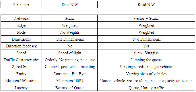
The data network and vehicular road network have different characteristics, features and hence a domain dependent approach is highly recommended.

Data network has speed of light, very high and hence longer travel path though add delays, is an option to consider whereas vehicle speed is lower by orders of several tens of magnitude than speed of light. Shortest path is computed based on distance, time to travel and driving comfort. One can define boundary conditions to limit the routes to be evaluated. Number of nodes in a city is far less than number of nodes in a data network leading to finite, manageable number of alternate routes. Domain Differentiation is an Advantage. Table 1 summarizes the comparison of features and enabling characteristics of the Data and road network.

Table 1. Feature comparison

4.3. Optimization

4.3.1. It is proposed to optimize the network to a manageable size to reduce the scope of the algorithm thereby reducing the processing time. Bounding Box is employed to limit the size of the network in terms of edges and nodes. The new network now is enclosed by bounding box between start and end nodes. Only the nodes embedded in this rectangle are considered, other nodes are ignored. Thus reducing computational requirements. There are two bounding box possibilities viz. Aligned to axis and Aligned to direction of the start & end node

4.3.2. Transport network nodes have latitude and longitude. Consideration of Lat / Long information of node increases algorithmic efficiency. The location coordinates in road transport network help in understanding if the approaching node is converging to the end node or not and correct intermediate node selection is made

4.3.2. There are three distances which play a role here: i) total distance between the two nodes under consideration; ii) distance to the target; iii) distance from the source. While approaching the end node, the decisive factor in selecting a node is minimal distance. The minimal distance is (Distance till node under consideration + Distance to the succeeding node to the target). A node may be connected to several edges leading to other nodes. Select a node with minimal distance.

4.3.3. Most importantly, city routes are a set of horizontal and vertical roads often converging to a junction. This makes the computation easier than the data network which diverges in different directions

4.3.4. In data networks, the data (entity) travels at speed of light which is not the case in road transport network

5. Representation, Iterations, & Algorithms

5.1. Representation

5.1.1. Graphical Representation

Below Figure 1 details the network with nodes represented with 2D coordinates and the edges having distances.

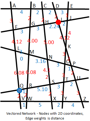Figure 1. Network with coordinate & edge lengths

5.1.2. Tabular Representation

Table 2 details the X & Y Cartesian coordinates for every node, it also lists distance of each node to a start node and end node depicted as D to Q and D to I, whereas Distance is the total distance of the node from start node to end node.

Table 2. Coordinates, Node Distances from start node, end node and summation of the two

5.2. Iterations – (Bi-Directional + Bounding Box)

The iterations and algorithm explanation is offered below for the same network mention above depicted through figure 2.

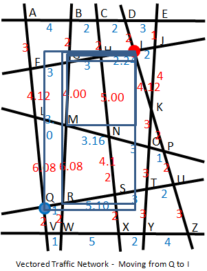Figure 2. Network with bounding box, Moving from Q to I

5.2.1. Moving from Start Node Q to End Node I

a. Start node Q

b. Create a bounding box

c. Q is connected to R only

d. R connects with M

i. (Distance from M to I + Distance from R to M) < (Distance from S to I + Distance from R to S)

ii. S is kept OPEN to be dealt later

e. M connects to G as N is out of bounding box

f. G connects to H

g. H connects to I

h. Route QRMGHI 16.32

OPEN S

a. Route so far QRS

b. S connects to N

c. N connects to H

d. H connects to I

e. Route QRSNHI 17.44

5.2.2. Moving from Start Node I to End Node Q is Depicted in Figure 3

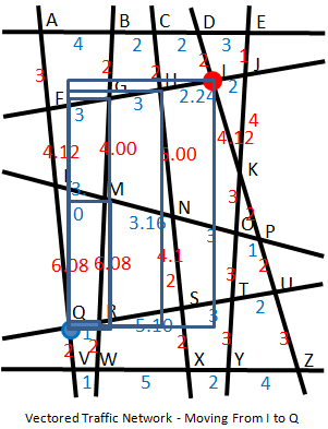Figure 3. Network with bounding box, Moving from I to Q

a. Start node I

b. I connects to H

c. H connects with N

i. (Distance from N to Q + Distance from H to N) < (Distance from G to Q + Distance from N to G)

ii. G is kept OPEN to be dealt later

d. N Connects to M as S is out of bounding box

e. M connects to R

f. R Connects to Q

g. Route IHNMRQ 17.48

OPEN G

a. Route so far IHG

b. G connects to M as N is out of bounding box

c. M connects to R

d. R connects to Q

e. Route IHGMRQ 16.32

5.3. Algorithm

1) Collect inputs

a. Start Mode

b. End Node

2) Initialization

3) Define a bounding box

4) Find connected Nodes

a. For every e = (E)

b. Compute nodes connected to edges in the bounding box

5) Find closest Node

a. For every v = (V)

b. Compute distance till succeeding node + distance from succeeding (node) to the destination node

c. Select minimum (d)

d. Store others in pending list

6) Repeat

a. Find connected nodes

b. Find closest node

7) Till pending list is nil

6. Proof of Concept / Result

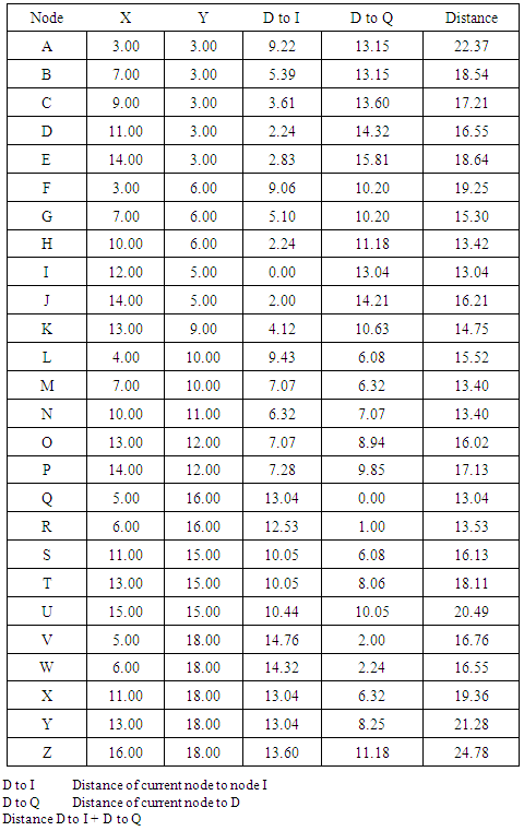
The shortest route exploration is done starting from both the ends Q as well as I. Starting from Q we get two shortest routes: Q R M G H I is 16.32 units and Q R S N H I is 17.44 units. Starting from I we get two shortest routes: I H N M R Q is 17.48 units and I H G M R Q is 16.32 units. It demonstrates that: From both the ends, we have consistent results. All the three results are feasible and consistent. The deviation from the shortest route offers alternate routes.

7. Congestion Analyses

7.1. Parameters

Time granularity is the sampling time interval. The permissible ratio of outflow to inflow rate is a decisive factor in building traffic congestion. All the directions are not GREEN Phased simultaneously and hence it is necessary to consider the green phase time and frequency in all the direction to arrive at an optimum ration. If the resultant outflow is less than inflow it is guaranteed congestion, if equal it can sustain present traffic load and if more than can accommodate higher traffic. There will be some vehicles present in each direction before starting the procedure.

7.2. Parameter Values

The simulation is done by setting different values of these parameters and observing the results. The priority is given to direction with maximum waiting vehicles. Time granularity 2; Vehicles present at the start in North, East, West and South directions is 50, 40, 30 and 20 respectively. Inflow rate is 5, 4, 3, and 2 from North, East, West and South direction respectively.

Case 1 Outflow to Inflow 3

The Outflow rate is based on the Outflow to Inflow ration and Inflow value is 20, 16, 12, 8 for North, East, West and South direction respectively.

Figure 4 shows the congestion is building continuously; Number of waiting vehicles in all the direction increasing. The time axes is same for all the directions where as the vehicle axes is different based on the number of waiting vehicles.

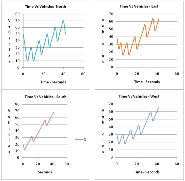Figure 4. Increasing congestion levels in North, East, South, West directions

Case 2 Outflow to Inflow 4

The Outflow rate is based on the Outflow to Inflow ration and Inflow value is 20, 16, 12, 8 for North, East, West and South direction respectively

Figure 5 shows the North direction stabilizes between maximum of 40 & a minimum of 10, the South between 33 & 20, the East between 32 & 8 and West between 36 and 18 vehicles.

Case 3 Finer granularity / Reducing the granularity

When the granularity is reduced, the sampling time is reduced and hence the decision to select the direction for green phase is taken immediately. This ensures there is even distribution of vehicles in all the direction over a period of time. However, the direction with minimum number of vehicles ends up starving for green phase as its green phase frequency is reduced. This can be balanced with flow rates.

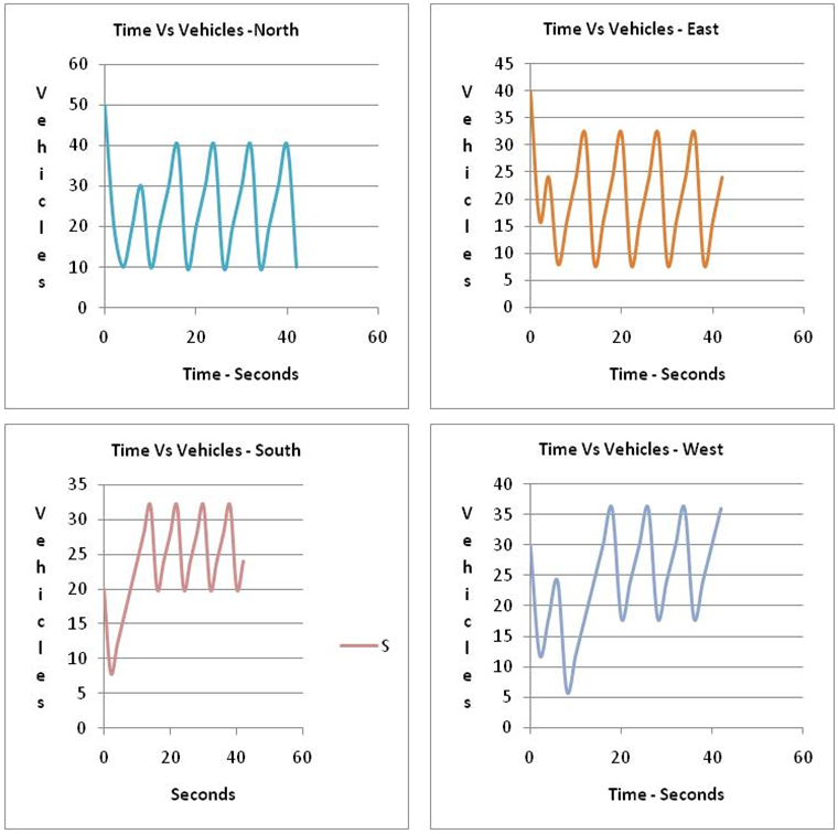Figure 5. Stabilized congestion in all the directions

8. Algorithm Comparison

Table three below compares the algorithms discussed before along with their performance.

Table 3. Algorithm comparison

Performance of these algorithms is proportional to the number of nodes and edges. Hence it is imperative that performance of these algorithms improve when subjected to less number of nodes for a given network.

Further let us consider a 8x8 network of 64 nodes. With two nodes (Light blue and dark blue) as start and end node.

Refer to Figure 6, a 8x8 node network will have 64 nodes and the algorithm will have to consider all the 64 nodes while computing the shortest route. If the same is optimized by a bounding box, it reduces to 36 node network, reducing the computation time by almost 50%.

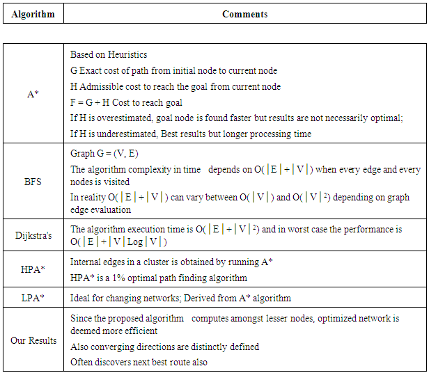
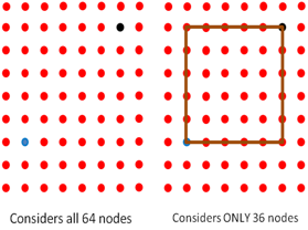Figure 6. 64 nodes network reduces to 36 node network

Refer to Figure 7, 64 nodes network is reduced to 18 node network thereby reducing the computation time by 70%.

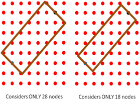Figure 7. 64 nodes network further reduces to 28 and 18 node network

9. Future Work

9.1. Traffic Offenses

9.1.1. Driving in One-Way

A vehicle travelling in the wrong direction / prohibited direction can easily be detected.

9.1.2. Wrong Parking

Vehicles parked in No-Parking zone can be detected. Long parking hours too can be detected which can lead to abandoned vehicle detection.

9.1.3. Jumping the Traffic Lights Detection is Easy Now

9.2. Collections

9.2.1. Zone based Toll

Cities are divided in two zones based on traffic congestion and hence zone based toll can be collected.

9.2.2. Pay-Per-Use Road Tax

Road tax too could be collected based on road usage by a vehicle.

9.3. Road Quality

Road quality could be evaluated easily. How many vehicles plied on the road before repair / reconditioning is required. Though it depends on the weight of the vehicle, a good beginning can be done and subsequently load cells can be installed at strategic points.

9.4. Post Accident Analyses

After accident takes place it is very difficult to reconstruct the exact movement of vehicles prior to the accident. The frame work will be able to provide speed and directions of vehicles prior to the accidents. Also hit-&-run cases too can be tracked easily.

9.5 Alternate Shortest Route

Shortest route has more traffic than other routes. This often leads the drivers to explore alternate shortest route. If there are N road segments in the shortest route, the alternate shortest route can be defined by replacing a minimum of 1 to maximum of N road segments. The road segments can be replaced by changing a single road segment, pair of road segment and so on.

Ideally, severity of traffic congestion in every road segment be evaluated and sorted in decreasing congestion severity. It is advised to have feasible alternate route for every road segment, pair of road segment and so on. In a city, driving habits, preferred routes do infuse shortest routes from the behavioral database. The system has knowledge database with history of travel for all the vehicles.