El-Sayed M. Ellaimony, Hilal A. Abdelwali, Jasem M. Al-Rajhi, Mohsen S. Al-Ardhi, Yousef Alhouli
Automotive and Marine Engineering Technology Department, College of Technological Studies, PAAET, Kuwait
Correspondence to: Hilal A. Abdelwali, Automotive and Marine Engineering Technology Department, College of Technological Studies, PAAET, Kuwait.
| Email: |  |
Copyright © 2015 Scientific & Academic Publishing. All Rights Reserved.
Abstract
Bicriteria multistage transportation problem without any restrictions in the intermediate stages is studied in this paper. We introduced an algorithm for solving this class of problems. The presented algorithm is based on dynamic programming technique with its capabilities to generate inherent parametric study during solution and techniques for solving bicriteria transportation problems. A way to find the non-dominated extreme points in the objective space is developed. This method involves a parametric search in the objective space. The dynamic programming technique is used to obtain the shortest route for transportation networks and methods for solving bicriteria linear programming. Our algorithm is applied to solve an illustrated example.
Keywords:
Transportation Problems, Multi-Stage Transportation Problem. Bi-Criteria Transportation Problem, Dynamic Programming
Cite this paper: El-Sayed M. Ellaimony, Hilal A. Abdelwali, Jasem M. Al-Rajhi, Mohsen S. Al-Ardhi, Yousef Alhouli, Solution of a Class of Bi-Criteria Multistage Transportation Problem Using Dynamic Programming Technique, International Journal of Traffic and Transportation Engineering, Vol. 4 No. 4, 2015, pp. 115-122. doi: 10.5923/j.ijtte.20150404.03.
1. Introduction
The classical transportation problem is the problem of obtaining the optimum distribution of certain commodities from several suppliers into several customers so that the total transportation cost becomes minimum [1, 2, 3]. It is investigated by many researches and known as Hitchcook Koopman transportation problem. In the traditional or classical transportation problem, the cost of transportation is directly proportional to the number of units transported. A lot of efficient algorithms had been developed for solving the transportation problems when the cost coefficients and the supply and demand quantities are known. The real world problems are multi-objective in nature. Most of the practical transportation problems appear with two objectives known as bi-criteria transportation problems. There are two objectives, minimization of total transportation cost and minimization of transportation time, or minimization of total deterioration.Deterioration is relevant in the case of certain perishable or decaying items. The degree of deterioration may depend on the route, mode and time of transportation. Clearly, this problem can be solved using any of the multi-objective linear programming techniques.Intensive investigations on multi-objective linear transportation problems have been made by several researchers. Aneja and Nair [4] presented an algorithm for solving bicriteria transportation problem using weighted sum method. A duality study for a linear multi-objective transportation problem is presented by Isermann [5]. Solving multi-objective transportation problem and an adjacent search is prepared by Diaz [6, 7]. Current et al [8] prepared a review of multi-objective design of transportation networks. Ringuest J.L. and Rinks D.B. [9] proposed the interactive solutions for linear multi-objective transportation problems.Practically, the transportation processes are done in many stages. The optimal solution for these problems depends on the nature of the problem and its network. Ivan Brezina and Adriana Istvanikova [10] presented a way of solving two-stage transportation problem. Al-Ellaimony E.E.M. [11] presented a mathematical model for all types of bicriteria multistage transportation problems. He presented both BMTP1, BMTP2, BMTP3, and BMTP4, and introduced a decomposition algorithm for solving BMTP3.In this paper we introduce an algorithm for solving BMTP1 which is a bicriteria multi-stage transportation problem without any transportation restrictions on the intermediate stages. The presented algorithm consists of three phases. Phases 1 and 2, determine both the minimum transportation cost and deterioration between the first stage sources and the last stage destinations. The dynamic programming technique is applied on these two phases using the shortest route procedure. Phase 3, determines the points of the non-dominated set in the objective space of the bicriteria transportation problem presented. The algorithm is presented by Aneja and Nair [4].
2. Different Forms of Bicriteria Multistage Transportation Problems [11]
The formulation of different bicriteria multistage transportation problems which are presented in this paper almost cover several real situation. The proposed formulations enable the decision maker discussing such transportation problems to find his goal.
2.1. Bicriteria Multistage Transportation Problems of the First Kind (BMTP 1)
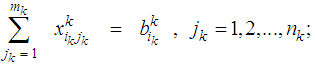
This case represents bicriteria multistage transportation problems without any transportation restrictions on the intermediate stages. In order to obtain the mathematical formulation of the problems representing this case let us assume that:cij = minimum transportation costs between the first stage sources and the last stage destinations.dij = minimum deterioration of a unit while transporting from first stage sources to last stage destinations.ai = Availabilities of the first stage sources.bj = Requirements of the last stages destinations.xij = Amounts transported from i to j.Then the problem takes the form: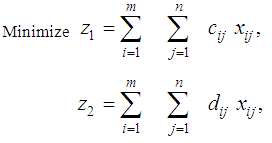 | (1) |
Subject to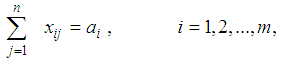 | (2) |
 | (3) |
2.2. Bicriteria Multistage Transportation Problems of the Second Kind (BMTP 2)
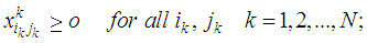
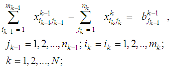
This case represents bicriteria multistage transportation problems in which the transportation at any stage is independent of transportation at the other stages.To obtain the mathematical formulation of the problems representing this case let us assume that, for Kth stage, K=1,2,…,N; the availabilities of the sources are  , ik=1,2,…,mk; the requirements at the destinations are
  , jk = 1,2,..,nk; the cost of transporting one unit from source (ik) to destination (jk) is
  ; and the deterioration of one unit while transporting from (ik) to (jk) is
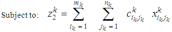
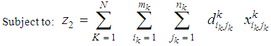
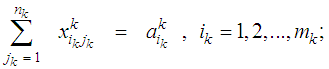
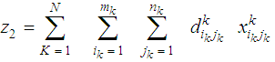
  .The mathematical formulation for this case can be written as (N) single stage bicriteria transportation problems in the form:
 | (4) |
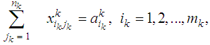
 | (5) |
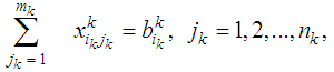
 | (6) |
 | (7) |
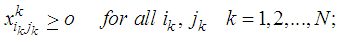 | (8) |
The minimum transportation cost and deterioration are given as: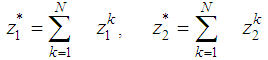 | (9) |
2.3. Bicriteria Multistage Transportation Problems of the Third Kind (BMTP 3)
This case represents bicriteria multistage transportation problems with some additional transportation restrictions on the intermediate stages which does not affect the bicriteria transportation problem nature at each stage.The mathematical formulation of the problem representing this case is given us: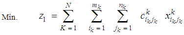 | (10) |
 | (11) |
 | (12) |
 | (13) |
 | (14) |
 | (15) |
Where: , k=1,2,…,N are linear functions representing the additional transportation restrictions at the (N) stages and, r is the umber of this linear functions at the kth stage.
2.4. Bicteria Multistage Transportation Problems of the Fourth Kind (BMTP4)
This case represents bicriteria multistage transportation problems in which the subtraction between the input and the output transportation commodity is known at the sources (destinations) of each intermediate stage. The assumed transportation restrictions in this case affect the transportation problem formulation of each individual stage.The mathematical formulation of the problem representing this case is given as: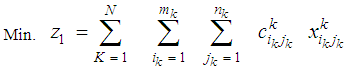 | (16) |
 | (17) |
Subject to: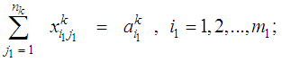 | (18) |
 | (19) |
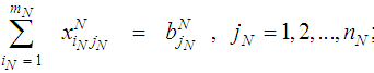 | (20) |
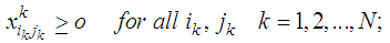 | (21) |
(BMTP1) Can be solved as a bi-criteria single stage transportation problem. This should be done after obtaining the shortest path between first stage sources and last stage destination. These routes represent the minimum cost coefficient and minimum deterioration coefficient between first stage sources and last stage destinations. So, the problem will be transformed into a bicriteria single stage transportation problem.(BMTP2) Can be solved as N bi-criteria single stage transportation problems. Then we can obtain the non-dominated solutions for each individual stage.(BMTP3) The decomposition technique can be used to solve this model to utilize the special nature of the transportation problems to determine the points of the non-dominated set in the objective space.(BMTP4) Can be solved using any algorithm for solving multiobjective linear programming problems.In this paper, we introduce an algorithm for solving bicriteria multi-stage transportation problem of the first kind (BMTP1). This algorithm uses the dynamic programming to find the shortest routes to transform the problem from multi-stage into a single stage transportation problem. The Aneja and Nair algorithm which is presented in [3] is used to obtain all of the non-dominated extreme points in the objective space for the studied case.
3. Dynamic Programming
Dynamic programming (D.P.) is a technique that can be used to solve many optimization problems. It is a useful mathematical technique for making a sequence of interrelated decisions. It provides a systematic procedure for determining the optimal combination of decisions. In most applications, D.P. obtains solutions by working backward from the end of a problem towards the beginning, thus breaking up a large unwieldy problem into a series of smaller, more tractable problems. D.P. divides problems into sub-problems called stages. After solving every sub-problem, the original problem solution can be achieved easily by using the state variables. State variables represent the links between stages which allow one to make optimum decisions for the remaining stages without having to check the effect of future decisions or decisions previously made. In other words, D.P. is based on a multistage decision process where a decision at one stage will affect the decision at subsequent stages. In contrast to other mathematical programming techniques, there does not exist a standard mathematical formulation for D.P. problems. But it is a general strategy for optimization rather than a specific set of rules. Consequently, the particular equation used must be developed to fit each problem. Abdelwali H. A. [12] introduced parametric multi-objective dynamic programming to solve some of automotive problems.The D.P. technique is applied in this paper to find the shortest route between all main sources in the first stage to all destinations in the last stage of the multistage transportation problem for all objectives. The shortest route here means the minimum transportation cost, and the minimum deteriorations from all sources in the first stage to all destinations in the last stage of the transportation network. With a transportation network of m-sources at the first stage and n-destinations at the last stage, we must find (m*n) shortest routes. In other words, we should have (m*n) shortest route problems we need to solve!The reason behind using D.P. to find these shortest routes and not using any other shortest route method comes from the fact that D.P. generates inherent parametric study for the problem solution. This inherent parametric study helps us to find the shortest route from any source to the last destinations. Another best advantage of these inherent results is reducing the number of computation required to find the shortest routes from all main sources to all last destinations from (m*n) problems into only n problems. For example, assume we have 12 main sources at the first stage, and 10 destinations at the last stage. To find the shortest routes from all main sources to all last destinations we need to solve 12*10= 120 problems. But only 10 problems (which equal the number of last destinations) can be solved using backward D.P. This reduces the time and effort required to find the shortest routes from all main sources to all last destinations.
4. Dynamic Programming Procedure Recursive Equation
4.1. Recursive Equation
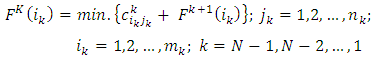
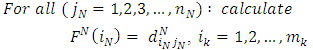
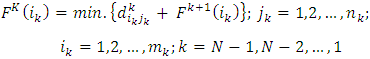
As mentioned above, the dynamic programming technique will be used to find the shortest route (where represent the transportations cost and deterioration) between all sources in the first stage to just one destination in the last stage. Then we need to repeat this procedure for all other destinations in the last stage. Of course this should be done for every single objective. So, the recursive equation for the backward dynamic program for the shortest route problem is illustrated in equations (22) to (25). Equations (22) calculate the minimum transportation cost to a certain destination from all the sources at the last stage. Equations (23) calculate the minimum transportation cost to all destinations from all sources at any other stage except the last stage. Equations (24) calculate the minimum transportation deterioration to a certain destination from all the sources at the last stage. Equations (25) calculate the minimum transportation deterioration to all destinations from all sources at any other stage except the last stage. 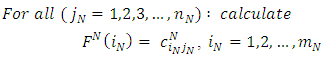 | (22) |
 | (23) |
 | (24) |
 | (25) |
Where: FN(iN): represents the optimum value of the studied objective for each source at the last stage (N).Fk(ik): represents the optimum value of the studied objective for each source at any stage except the last stage.K: stage number, k= 1,2,3,..., K : transportation cost at the last stage (N) from its sources iN to its destinations jN.
 : transportation cost at any stage (k) from its source ik to its destinations jk.
 : transportation deterioration at the last stage (N) from its sources iN to its destinations jN.
 : transportation deteriorations at any stage (k) from its source ik to its destinations jk.iN: the source number at the last stage (N).jN: the destination number at the last stage (N).ik: the source number at any stage (k) except the last stage.jk: the destination number at any stage (k) except the last stage.mN: the total number of sources at the last stage (N).nN: the total number of destinations at the last stage (N).mk: the total number of sources at stage (k).nk: the total number of destinations stage (k).
4.2. Solution Algorithm
There are two algorithms exist in this paper. The first solution algorithm includes two phases (phase 1 and phase 2). This algorithm is used to find the minimum transportation costs and the minimum deteriorations between the first stage sources and the last stage destinations. This transforms the problem from bicriteria multi-stage into bicriteria single stage transportation problem. The second algorithm is summarized in (phase 3) to obtain the set of nondominated extreme points for the single stage bicriteria transportation problem which is generated from algorithm number 1.
4.2.1. Phase 1
Step 1: Set jN = 1.Step 2: Use the recursive equations (22) to obtain the transportation cost (FN(iN)) between all sources (iN = 1,2,…mN) to destination number (jN) at the last stage. Step 3: Use the recursive equations (23) to obtain the minimum transportation cost (Fk(ik)) between all sources (ik= 1,2,…mk) to all destinations for all stages (K= N-1, N-2, … 1).Step 4: If (jN = nN), go to phase 2. Otherwise, set (jN = jN+1) then go to step 2 of this phase 1.
4.2.2. Phase 2
Step 1: Set jN = 1.Step 2: Use the recursive equations (24) to obtain the transportation deterioration (FN(iN)) between all sources (iN = 1,2,…mN) to destination number (jN) at the last stage. Step 3: Use the recursive equations (25) to obtain the minimum transportation deterioration (Fk(ik)) between all sources (ik = 1,2,…mk) to all destinations for all stages (K= N-1, N-2, … 1).Step 4: If (jN = nN), go to phase 3. Otherwise, set (jN = jN+1) then go to step 2 of this phase 2.
4.2.3. Phase 3
This phase determines the nondominated extreme points in the objective space for a bicriteria single stage transportation problem obtained from phases (1) and (2). The algorithm is validated by the following theorem [4].4.2.3.1. TheoremA point 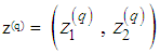 is a nondominated extreme point is the objective space if and only if z(q) is recorded by the algorithm. 4.2.3.2. Step 1: For bicriteria single stage transportation problem, find
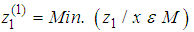 And find
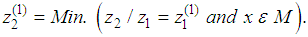
 Similarly, find
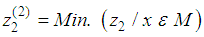 And find
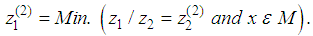
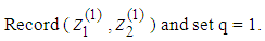
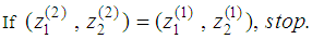 Otherwise record
  and set q = q+1Defines sets L = {(1,2)} and E = , and go to step 2.4.2.3.3. Step 2: Choose an element (r, s) ∈L and set
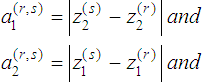 Obtain the optimal solution
  to the transportation problem.
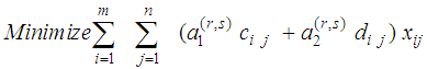 Subject to:
 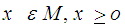 If there are alternative optima, choose an optimal solution
  , for which
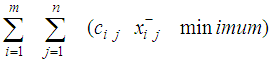 Let:
Let: 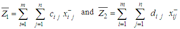 If
If  is equal to
  Set
Set  and go to step 3.Otherwise record
  such that
 and go to step 3.4.2.3.4. Step 3:Set L = L - {(r-s)}. If L = , stop.Otherwise go to step 2.
5. Illustrative Example
5.1. The Problem
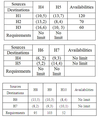
We applied the presented algorithm to solve a simple 3-stage bicriteria transportation problem of the first kind (BMTP 1). The chosen 2-objectives are transportation cost and deteriorations. Figure 1 below represents this simple network. The availabilities of the main sources at stage 1 equals are those values of (a1, a2 and a3). The requirements of the destinations at the last stage are those values of (b1, b2 and b3). There are no transportation restrictions on the middle stages availabilities or requirements. The values of both the transportation unit costs and the deterioration amount while transporting the product from any source (ik) to any destination (jk) through a certain stage (k) is illustrated on the arcs as 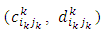 . It is required to find the non-dominated set of extreme points for this problem. All the problem data are included in Tables (1, 2 and 3) below. All these data are summarized in Table (1).
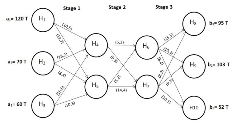 | Figure 1. The illustrative example network |
Table 1. Cost and deterioration of transportation & availabilities and requirements for stages (1, 2 and 3) resp
 |
| |
|
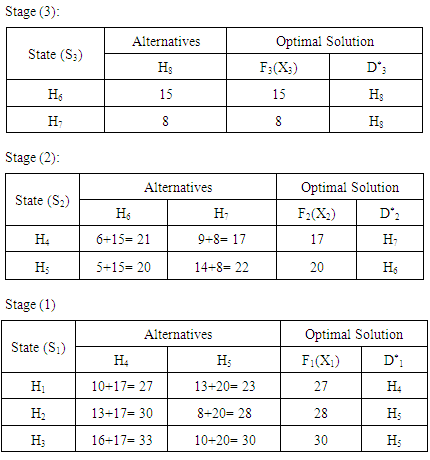
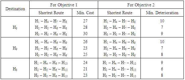
5.2. Dynamic Programming Results
Since we have 3 destinations in the last stage of this example, therefore, we need to solve 3 D.P. problems for each objective. So, the first step to solve this problem is to apply phase (1) and phase (2) in the solution algorithm to find the minimum transportation costs and the minimum deteriorations from all sources of the first stage to all destinations of the last stage. Then we use these results to convert the 3-stage network into a single stage problem. Table (2) below shows the D.P. stages to find the shortest route, for just problem, for the first objective (the transportation cost) from all sources of the first stage (nodes: H1, H2 and H3) to node (H8) only at the last stage. This same procedure is applied to find the shortest route from (H1, H2, and H3) to both (H8, H9 and H10) for both objectives. Table (3) summarizes the shortest route for all other problems for both objectives. Figure 2 illustrates the equivalent single stage transportation problem according to D.P. results. Both cij and dij values are in dollars/ton.kilometer. The values of Xij are in ton.kilometer. 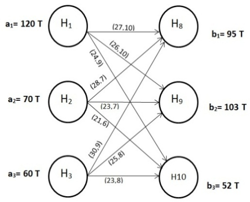 | Figure 2. The equivalent network |
Table 2. Dynamic Programming Stages To Find The Shortest Routes From (H1, H2 and H3) To (H8)
 |
| |
|
Table 3. D.P. results for all problems of the 2 objectives
 |
| |
|
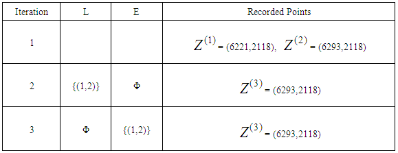
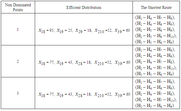
5.3. Bicriteria Phase (3) Results
Phase 3 is then applied on the new equivalent problem to determine the efficient distribution and the non-dominated extreme points accompanying each iteration, the minimum transportation cost and minimum deterioration as single objective problems. The results are summarizes in Tables (4) and (5). The decision maker should Choose a non-dominated point and its related distribution from Tables (4), and (5) according to his/her point of view.Table 4. Solution of the illustrative example in the objective space
 |
| |
|
Table 5. Non dominated solutions and the related efficient points
 |
| |
|
6. Conclusions
In this paper, we introduced 2 solution algorithms in 3 phases to solve the bicriteria multistage transportation problem of the first kind (BMTP1). The presented algorithms enable solving such problems more realistically to find all efficient extreme points. The bi-criteria multi stage transportation problem can be solved using the standard technique of a transportation problem.Dynamic programming is a very powerful technique to reduce the multi-stage into a single stage transportation problem, when there are no restrictions in the middle stages sources availabilities and destinations requirements point of view. The decision maker then, will get all non dominated solutions with their efficient points and their related distributions. Therefore, s/he can choose any point from the non dominated solution which meets his/her requirement.
References
| [1] | Frederick Hillier, Introduction to Operations Research, with Student Access Card, Edition 10th, McGraw-Hill, 2014. ISBN-13: 978-1259162985 ISBN-10: 1259162982. |
| [2] | Taha H.A., Operations Research, An Introduction, 9th Edition, Prentice Hall, 2010. ISBN-13: 978-0132555937 ISBN-10: 013255593X. |
| [3] | Sang M. Lee and David L. Olson, Introduction to Management Science, 3e Paperback, Edition 3rd, Cengage Learning, 2005. ISBN-13: 978-0324415995 ISBN-10: 0324415990. |
| [4] | Aneja Y.P., Nair K.P.K., Bi-criteria transportation Problems, Management Science, 1979, vol. 25, pp 1 – 11. |
| [5] | Isermann H., The enumeration of all efficient solutions, Naval Research Logistic Quarterly 1979, vol. 26, pp 123 – 139. |
| [6] | Diaz J.A., Solving multi-objective transportation problem, Ekonomicko- Matematicky Obzor, 1978, vol. 14, pp 267 – 274. |
| [7] | Diaz J.A., Finding a complete description of all efficient solutions to a multi-objective transportation problem, Ekonomicko- Matematicky Obzor, 1979, vol. 15, pp 62 – 73. |
| [8] | Current J., Min H., Multi-objective design of transportation networks: Taxonomy and annotation, European Jornal of Operations Research, 1986, vol. 26. |
| [9] | Ringuest, J.L., Rinks, D.B., Interactive solutions for the linear multiobjective transportation problem, Eur. J. Oper. Res. 32, 1987, 96 – 106. |
| [10] | Berzina, Istranikova, The way of solving two-stage transportation problems, Mathematical Methods in Economics 1999, 39 – 44. |
| [11] | Ellaimony E.E.M., Different Algorithms for Solving Multi-Stage Transportation Problems, Ph.D., Helwan University, Egypt, 1985. |
| [12] | Abdelwali H.A., On Parametric Multi-Objective Dynamic Programming With Applications To Automotive Problems, Ph.D., El-Minia University, Egypt, 1997. |
 Abstract
 Reference
 Full-Text PDF
 Full-text HTML