Jaehoon Kim1, Michael Anderson1, Sampson Gholston2
1Civil & Environmental Engineering, University of Alabama in Huntsville, Huntsville, USA
2Industrial & Systems Engineering and Engineering Management, University of Alabama in Huntsville, Huntsville, USA
Correspondence to: Jaehoon Kim, Civil & Environmental Engineering, University of Alabama in Huntsville, Huntsville, USA.
| Email: |  |
Copyright © 2015 Scientific & Academic Publishing. All Rights Reserved.
Abstract
The Highway Safety Manual, 1st Edition (HSM), was released in 2010, which provides analytical tools and techniques to estimate expected crash frequencies for various roadway facilities. After the release of the HSM, a large amount of HSM calibration research has been conducted to adapt to individual jurisdictions. Even with the amount of research, there are still some challenges to applying the HSM due to lack of data. The data required is obtained from Critical Analysis Reporting Environment (CARE) the data analysis software package developed by the Center for Advanced Public Safety (CAPS) at the University of Alabama. The goal of this study was to conduct calibration of SPFs for urban and suburban arterials in the HSM. Initially, the development of a calibration factor (C-factor) using the HSM guideline was performed. Then, an estimate proper sample size was developed. Finally, statistical modeling is performed using jurisdiction crash data and the negative binomial (NB) regression model to estimate Alabama-specific SPFs, including a model validation to examine statistical model fit.
Keywords:
Safety Performance Function, Calibration, Statistical Modeling
Cite this paper: Jaehoon Kim, Michael Anderson, Sampson Gholston, Modeling Safety Performance Functions for Alabama's Urban and Suburban Arterials, International Journal of Traffic and Transportation Engineering, Vol. 4 No. 3, 2015, pp. 84-93. doi: 10.5923/j.ijtte.20150403.02.
1. Introduction
The Highway Safety Manual, 1st Edition (HSM), was released in 2010. The HSM consists of the crash frequency prediction models of various types of road facilities, and provides analytical methods, tools and techniques for quantifying the potential crash risk. However, the HSM has limitations in its predictive method, Part C, due to differences in jurisdiction. The safety performance functions (SPFs) were developed using limited data based on selected states. It is possible that the results of estimation could be significantly biased or different with the actual crash frequency. Therefore, the HSM recommends calibration of the model to increase the accuracy and to get valid prediction results from the HSM (AASHTO 2010). However, HSM users, such as state Department of Transportation (DOT) or other institutions, do not have the necessary data that corresponds to the HSM requirements or do not have well organized accident information and geometry data. Even though the Center for Advanced Public Safety (CAPS) at the University of Alabama developed an accident database named Critical Analysis Reporting Environment (CARE) in Alabama, it is not possible to directly apply this database on the HSM methodology due to lack of information. The CARE data consists of 0.01 mile roadway segment and each segment contains ninety-one variables including traffic volume, highway functional class, total crash frequencies, frequencies of each type of crash, and many other roadway variables. The CARE data consists of multiple-vehicle collision and single-vehicle collision data; however, there is not data for drive-way collisions. Also, the roadway inventory does not include the number of driveways on each segment. Therefore, it is not possible to directly apply HSM SPFs to the state of Alabama. The goal of this study was to conduct calibration of SPFs for urban and suburban arterials in the HSM. Unlike other Safety Performance Functions, (SPFs), the SPFs of urban and suburban arterials contain numerous formulas. The important elements of the formulas include: (1) the function of multiple-vehicle collisions, (2) the function of single-vehicle collisions, and (3) the function of driveway collisions. For the safety analysis of the roadway facilities, the number of accidents with roadway information is required. We firstly develop the calibration factor (C-factor) using the HSM guideline, which is to calculate the ratio of the actual crash frequency to the predicted crash frequency. Then, we estimate proper sample size. We also performed statistical modeling using jurisdiction crash data. Particularly, negative binomial (NB) regression model was used to estimate Alabama-specific SPFs. In addition, this study conducts model validation to examine statistical model fit.
2. Literature Review
The first version of the HSM, published by the American Association of State Highway and Transportation Officials (AASHTO) in 2010, provides analytical tools and techniques to estimate expected crash frequencies of various types of roadway facilities. In Part C of HSM, predictive methods and procedures are provided. The predictive methods in the HSM offer safety performance functions (SPFs) as a quantitative measure for estimating expected crash frequencies an ideal conditions. The procedure of estimating the number of crashes consists of 18 steps. To sum up, the predicted average number of crash is estimated under each type of facility. After the estimation, Crash Modification Factors (CMFs) and calibration factor C is calculated and applied in the estimation (AASHTO 2010). SPFs are regression functions of annual average daily traffic (AADT) and length of the segment to estimate crash frequency for a particular roadway facility type (AASHTO 2010). SPFs are based on negative binomial (NB) distribution because NB regression model is more appropriate to estimate count response and can handle over-dispersion (AASHTO 2010) (Lord and Mannering 2010). CMFs are the ratio of the real condition to the ideal condition at a site. CMFs are multiplied by the ideally estimated crash frequency predicted by SPFs in HSM to adjust the differences between the ideal conditions and practical conditions (AASHTO 2010). NB model is frequently used in research to predict crashes on the highway facilities. Specifically, when the crash data shows over-dispersed distribution, NB regression model is an appropriate statistical model for predicting crash frequency (Lord 2006). The NB regression model is, the extended model of the Poisson model, to overcome over-dispersion problem in the crash data. Over-dispersion means that the variance exceeds the mean of the data. Generally crash count data exhibits over-dispersed distribution. The over-dispersion problem may lead the Poisson model to result in a biased estimation (Lord and Mannering, The Statistical Analysis of Crash-Frequency Data: A review and Assessment of Methodological Alternatives 2010). Many state agencies and/or researchers in academia have conducted HSM calibration research on various facilities. Michigan Department of Transportation (MDOT) conducted calibration research for all of facilities in the HSM, freeway segment and interchange. MDOT calculated the calibration factors of total crashes and all injury crashes for each of the five study years (Michigan Department of Transportation 2012). Srinivasan (Srinivasan and Carter 2011) calibrated SPFs for six of roadway segment types and eight types of intersection facilities in North Carolina. They used the Highway Safety Information System, NCDOT GIS files, Google aerial and Streetview imagery data. Sun et al. (Sun, et al. 2013) calibrated HSM predictive models for various types of roadway facilities including freeway segments. They collected the data for the calibration from a variety of sources, such as MoDOT transportation management system database and Google imagery data. Shin et al. (Shin, Lee and Dadvar 2014) developed local calibration factors in Maryland. Their focus of calibration includes eight types of roadway segments and ten types of intersection facilities. Srinivasan et al (Srinivasan, et al. 2011) calibrated the SPFs of HSM for both segment and intersection level. The authors assumed some elements such as driveway density, roadside hazard rating, and fixed objects, due to lack of information. Therefore, this study also performed the sensitivity analysis in order to examine the impact of Srinivasan et al (2001)'s assumptions. Williamson et al. (Williamson and Zhou 2012), Xiao et al. (Qin, Chen and Vachal 2014), Lubliner et al. (Lubliner and Schrock 2012), and Brimley et al. (Brimley, Saito and Schultz 2012) conducted Two-lane Two-way roadway HSM calibration for other states. Their research mostly used the calibration methodology, which is recommended by the HSM to compute the calibration factor. On the other hand, the state of Virginia (Kweon, et al. 2014) and the state of Louisiana (Sun, et al. 2011) undertook the calibration research of the rural multilane highways. Virginia DOT also developed the guidance for application and calibration of HSM for Virginia. In Oregon, Fei Xie et al. (Xie, et al. 2011) conducted the calibration studies for all of the facilities in Oregon. Fei Xie et al. (2011) developed and provided a new regressions models to estimate the number of pedestrian and minor road AADT due to difficulties in collecting data in Oregon. Their models can be helpful to overcome data collection deficiency. Kansas developed a linear calibration method to focus on animals due to crashes because a large amount of crashes related animal occurred in the state. Brown et al. (Brown, Sun and Edara 2013) described the empirical approaches and discussed some challenges faced during the research. Vanvi Trieu et.al. (Trieu, Park and McFadden 2013) performed a sensitivity analysis to find the appropriate number of samples and to calibrate Two-lane Two-way undivided urban arterials in New Jersey. To find the ratio of calibration factor, the authors conducted Monte-Carlo simulation with 500 iterations. When 50 percent of samples or more were selected, the ratio of the calibration factor had a margin of plus or minus 5 percentage points (Trieu, Park and McFadden 2013). Persaud et. al. (Persaud, et al. 2012) focused on two applications of the HSM predictive methods for Canadian highways. The study assessed the HSM algorithm for urban signalized intersections in Toronto and developed Canada jurisdiction-specific SPFs. The last study that performed urban area facility calibration is Oregon state HSM calibration. Mehta and Lou (Mehta and Lou 2013) have conducted the Two-lane Two-way rural roadways SPFs calibration study for the state of Alabama. The authors adopted various prediction models from other studies as well as developing the SPFs specifically for Alabama.
3. Data Preparation
3.1. Data Description
The data used in this study was obtained from the Critical Analysis Reporting Environment (CARE) developed by the Center for Advanced Public Safety (CAPS) at the University of Alabama. CARE includes analytical and statistical tools to produce appropriate information directly from the raw data (CENTER for ADVANCED PUBLIC SAFETY 2014). The data contains 192 total variables including the number of vehicles related the accident, number of pedestrians related to the accident, type of the vehicle crash, etc. For this study, CAPS provided the special data extracted from the original CARE data. The data consists of 0.01 miles roadway segments representing 1,365.55 miles of urban area roadway. Each segment contains ninety one variables including AADT, highway functional class, total crash frequencies, frequencies of each type of crash, the presence of median, median type, the presence of Two-Way Left Turn Lane (TWLTL) and other requisite information. The study used the available data sets for years from 2007 to 2009.
3.2. Integrating Homogeneous Roadway Segments
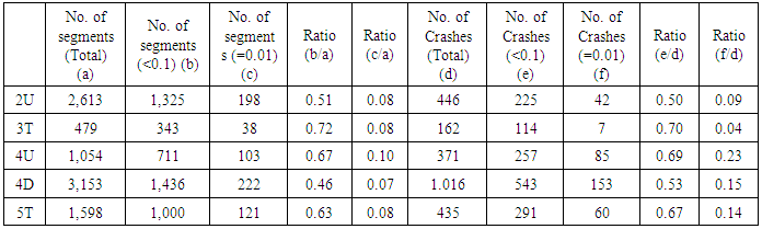
The CARE data consists of 0.01 mile roadway segments, so that the roadway segments should be merged into homogeneous sites to perform calibration study. Generally, each roadway segment begins at the center of one intersection and ends at the center of the next intersection, or it consists of one homogenous segment followed by another homogenous segment. Each homogeneous site should have the same geometry design features and traffic control characteristics. Therefore, we set the main variables to integrate each segment into a homogeneous site. The main variables used in this step are AADT, the number of lanes, median type, median width, presence of TWLTL, presence of an intersection, and speed limit. After integrating the segments, we create 9,999 homogeneous roadway segments. The next step is to divide each type of roadway facility. In the HSM, urban and suburban roadway facilities are classified as Two-lane undivided arterials (2U), Three-lane arterials including a center two-way left-turn lane (TWLTL) (3T), Four-lane undivided arterials (4U), Four-lane divided arterials (4D), and Five-lane arterials including center TWLTL (5T). Considering the characteristics of the facilities, we categorized 9,999 homogeneous segments by the five types of facilities. As a result of the step, we created 2,613 sites of 2U, 479 sites of 3T, 1,054 sites of 4U, 3,153 sites of 4D, and 1,598 sites of 5T. Six or more lanes facilities are eliminated because the HSM does not address those types of facilities in this edition. The integration procedure was automatically computed using Visual Basic Application script of Excel.The minimum length of the segment is 0.01 mile and the maximum length of segment is 2.14 mile. The average length of each segment was approximately 0.14 mile. The HSM mentioned that there was no minimum roadway segment length, but 0.10 mile of segment length for minimum decreased the burden of data collection and calculation effort (AASHTO 2010). Srinivasan et al. (Srinivasan, et al. 2011) used 0.04 mile for urban and suburban segments as minimum value. The other segments shorter than the minimum were not used in the calibration study in Florida. Also, Shin et. al. (Shin, Lee and Dadvar 2014) stated that the minimum length of 0.1 mile suggested by the HSM is too long in Maryland because more than 80 percent of urban and suburban arterials are shorter than 0.1 mile. In Alabama, more than 50 percent of urban arterials are shorter than 0.1 mile, and approximately 8 percent of segments have 0.01 mile length. In addition, more than half of crashes occurred on the segments which are shorter than 0.1 mile, and more than 10 percent of total crashes occurred on the 0.01 mile length segments. Therefore, this study include all of the segments to perform the calibration study.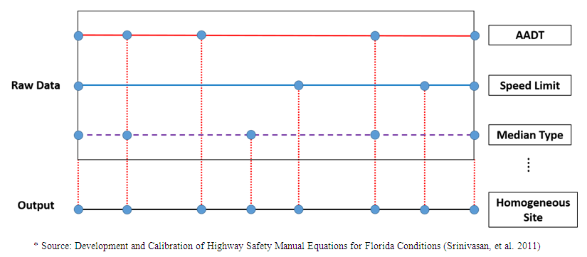 | Figure 1. Homogeneous Segments Development |
Table 1. Data Description

 |
| |
|
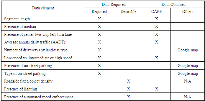
Table 2. Data Requirement
 |
| |
|
3.3. Site Selection
Focusing on the calibration of urban and suburban arterial in the HSM predictive methods, the HSM recommends that thirty to fifty segments, which are used in calibration process, are required to estimate the expected average crash frequency (AASHTO 2010). In the previous step, homogenous segments are merged according to the key attributes that affect SPFs and/or CMF, and each type of urban and suburban arterial was classified with the HSM criteria. HSM and most of the previous calibration studies recommended random selection of the sites to avoid site selection bias. This study randomly and independently selected fifty sites from that developed data sets for each year. There are several limitations to directly apply the CARE data on the HSM methodology: no information of density of driveways, limited information of adjacent land use of the segment, no information of the presence of on-street parking and the type of the parking. Therefore, we collected the missing data manually using the Google map. The estimation of expected average crash frequency in this research was limited to urban and suburban arterials in Alabama. The required data to estimate predicted crashes are showed in the below table.
4. Methodology
4.1. Safety Performance Functions (SPFs)
The SPFs for urban and suburban arterials in HSM are more complicated than the SPFs for rural area arterials. The predictive methods for urban and suburban roadway segments consist of three negative binomial regression models basically, of which AADT and length of roadway segment, and various functions with multiplicative factors. The general form of predictive models to forecast average crash frequencies in this study is shown below : | (1) |
 | (2) |
 | (3) |
 | (4) |
 | (5) |
 | (6) |
 | (7) |
 | (8) |
 | (9) |
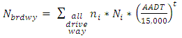
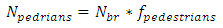
Unlike other SPFs of roadway facilities, the SPFs for urban and suburban arterials contain various formulas. The important functions of the formulas can be emphasized as: (1) the function of multiple-vehicle collisions, (2) the function of single-vehicle collisions, and (3) the function of driveway collisions. The entire process to calculate the predicted crashes is based on these three functions. The sum of the result of these three functions is the fundamental result of expected crashes of only vehicles on each segment. The expected crash frequency related to pedestrians and the bicycles are proportions of predicted average crash frequency of vehicles only.
5. Estimation Result
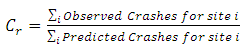
In this step, we developed the C-factor using the methodology provided by HSM. HSM provides the calibration guideline that involves five steps of the calibration procedure and data requirements. However, some of the HSM`s requirements are not suitable to apply to the CARE data in Alabama. HSM recommends that 30 to 50 sites are required to perform a calibration study. Also, those selected sites should be randomly selected, and represent at least 100 accidents per year. However, this requirement cannot be applied Alabama. Table 3 shows the number of roadway segments, total accidents of three years, and average accidents per segment. For example, random sampling process was performed more than 100,000 for all of the facility types. Only 4D reached the minimum accident constraint, the others could not. It indicated that the minimum accident frequency should vary depending on the accident rate in the study area.Table 3. Statistics of Roadway Segments
 |
| |
|
Thus, we prepared two scenarios depending on the number of sample sites. The first scenario was to perform the calibration procedure with 50 sites without the consideration of minimum accident frequency. Using CARE data, collected data, and uncalibrated SPFs of HSM, we calculated the expected average crash frequency of each type of urban and suburban arterial.
5.1. Urban and Suburban SPFs Calibration
5.1.1. First Scenario
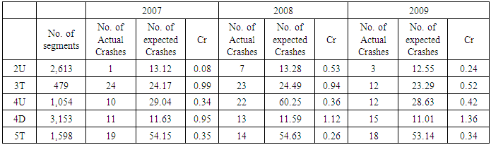
Table 4 shows the actual crash frequency, predicted crash frequency, and C-factor during the three years between 2007 and 2009. The C-factors show significant differences between each year in 2U. In addition, relatively too low C-factors can be detected, and the number of actual crash history is also varies.Table 4. Results of the Calibration
 |
| |
|
5.1.2. Second Scenario
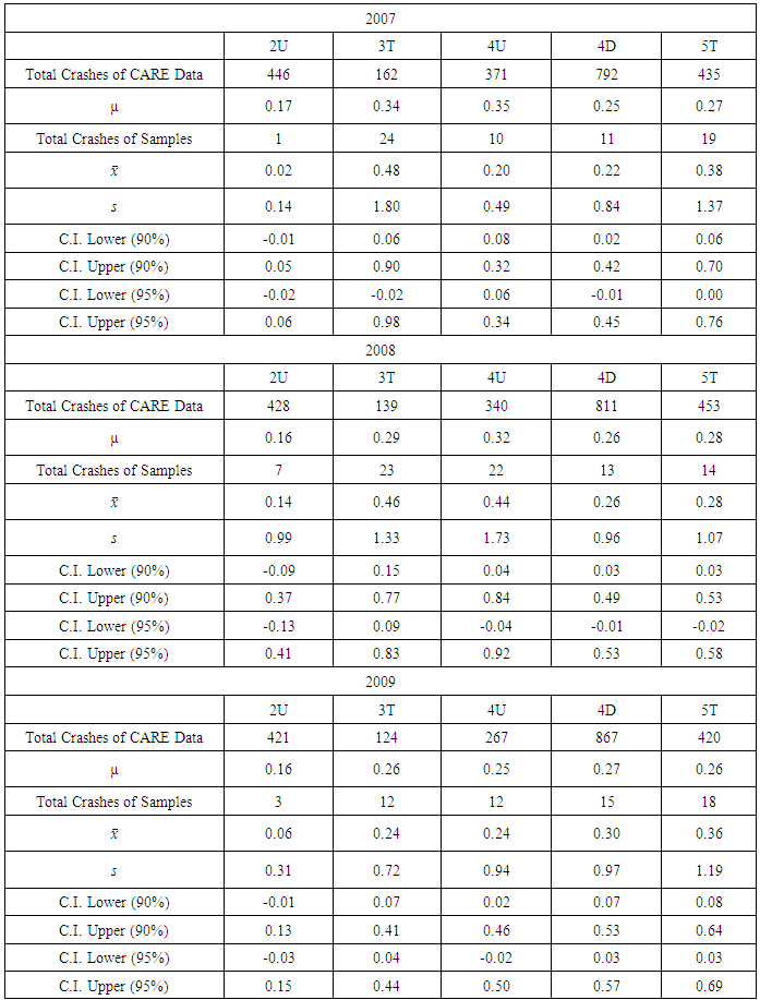
The second scenario was to estimate proper number of samples to conduct the calibration study. Firstly, we construct 90% and 95% confidence intervals (CI) on the population mean. If the population mean is not within the CI, we can conclude that the 50 samples came from a population with a different mean. As a result of the test, sample means of 2U and 4U are not within the both of the CI in 2007, and 2U sample mean is not statistically significant with 90% and 95% CI in 2009. Therefore, it is required to find proper sample size to perform the calibration study (see Table 5). Table 5. Results of Confidence Interval
 |
| |
|
Even though HSM mentioned 30 to 50 samples are sufficient to collect data, 50 samples are not enough to represent the Alabama accident characteristics. Shin et. al. (Shin, Lee and Dadvar 2014) applied the following equation to calculating sample size,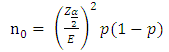 | (10) |
 | (11) |
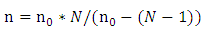
where n represents the minimum sample size, N is the number of population, n0 is the initial sample size, Z represent area under normal curve, 100(1-α) represents the confidence level, p is true proportion, and E is margin of errors. We assume margin of errors is 10% and 20% the of population mean by each facility, and the confidence level is 90%.Table 6. Results of Calculating Sample Size
 |
| |
|
The estimated sample size has significantly increased than 50.
5.2. Estimation of the Safety Performance Function
This step was to develop jurisdiction-specific SPF for multiple-vehicle collision using Alabama CARE data. Two subsets of the CARE data, which are developed in the previous step, are used in this development procedure. CARE data consists of single-vehicle collisions and multiple-vehicle collisions. As mentioned above, CARE does not contain important information related to the driveways density in the geometry data and in the accident data. Therefore, it was not possible to specify the number of crashes related to the driveways. For the reason, we attempted to develop the Alabama-specific model for the multiple-vehicle collisions and the single-vehicle collisions.
5.2.1. Multiple-Vehicle Collision SPF
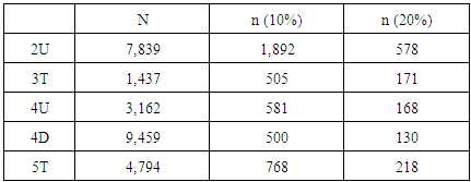
According to the previous studies of the development of crash estimation models, most of the variables were included in the initial model such as AADT, segment length, lane width, shoulder width, and on-street parking. The final model includes only AADT and the length of segment as the independent variables. In this study, we develop three types of the SPFs. The functional forms are not significantly different with the SPFs of the HSM. However, we directly applied AADT on the conventional NB regression model as a predictor. Generally, log-transformed AADT is used as the main independent variables in HSM and other previous studies. The reasons are not only that researchers attempt to experiment with a different model form, but also that the log-transformation can reduce the skewness of AADT data (Brimley, Saito and Schultz 2012). The first model is the same model form with HSM including log-transformed AADT as a predictor and a segment length as an exposure variable. The second model is a conventional negative binomial regression model including AADT and segment length as independent variables. The last model is a NB regression model including AADT as an independent variable and segment length as an exposure variable. The SPFs of urban and suburban arterials for the multiple-vehicle collisions are developed with the statistical analysis software STATA (LPStataCorp, STATA 13 2014). | (12) |
 | (13) |
 | (14) |
The estimated coefficient and constant values of the regression models are summarized in the following table.Table 7. Estimated Parameters for SPFs of Multi-Vehicle Collisions
 |
| |
|
5.2.2. Single-Vehicle Collision SPF
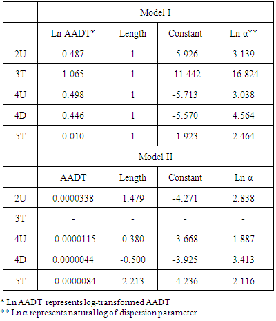
According the NCHRP report (Harwood, et al. 2007), the single-vehicle collision SPF uses the form of the multiple-vehicle collision SPF because the researchers did not find statistically significant models for single-vehicle collisions for all cases. Also, the NCHRP research attempted to develop single-vehicle collision as a simple function using multiplicative factor because there is no formal model available. In addition, using only multiplicative factor, the AADT would not affect dependent variable. Therefore, we simply estimate the coefficients of the independent variables and an intercept using Model form I and II of multiple-vehicle collisions from the previous step. | (15) |
 | (16) |
Table 8. Estimated Parameters for SPFs of Single-Vehicle Collisions
 |
| |
|
6. Model Fit Test and Model Validation
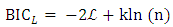
A statistical model was required to check the analysis of model fit. There are many types of model fit test such as the R2 or pseudo R2 goodness of fit, the deviance goodness-of fit, or the likelihood-ratio test. In this study, we use information criterion tests, the Akaike Information Criterion (AIC) and the Bayesian Information Criterion (BIC). This is because the models estimated in this study are calculated based on maximum likelihood estimation and the AIC statistic is related to the model log-likelihood. The BIC is another model fit test method for likelihood-based statistical models. Both the AIC and BIC indicate that comparatively lower value means a better fitted model (Hilebe, Negative Binomial Regression 2011). | (17) |
where  is the log-likelihood of the model, and K is the number of parameters.
 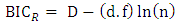 | (18) |
 | (19) |
where D is the model deviance and d.f is the degrees of freedom. The n represents sample size, and the k indicates the number of parameters. The BICR and BICL have different value, but for both, the higher value is usually given in statistics softwares. It is recommended that the data for validation should not include the data used in the modeling procedure, and it should be selected from same population, or the validation data can be sampled from the data used in the model. Generally 20 percent of data are extracted (Hilebe 2011). In this validation, we set a validation data in the previous step. Half of the total data is used to estimate the statistical models, and the remains are used in the validation step. Two model performance measures: (1) Mean Prediction Bias (MPB) and (2) Mean Absolute Deviation (MAD), are used to assess model performance. For the validation, validation part, they are prepared as distinct from the modeling data set.
6.1. Mean Prediction Bias (MPB)
The MPB is a measure of the direction and the magnitude of bias measured by comparing observed values and expected values in the validation data. A positive value indicates that a regression model overestimates crash frequency and vice versa. The magnitude of a value indicates the average prediction bias, and smaller absolute values represent better model to predict crash frequency.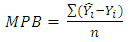 | (20) |
where  = the predicted value of
  , and n = sample size of validation data
6.2. Mean Absolute Deviation (MAD)
The MAD is the measure of difference between observations and predicted values. It is different from that of MPB because the negative and positive values between the observations and predictions do not cancel each other. The prediction errors are represented as positive values, and when the result of MAD is close to zero, it indicates that the prediction model provides better result . 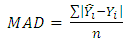 | (21) |
6.3. Results of the Fit Test and Validation of SPFs for Multiple-Vehicle Collision
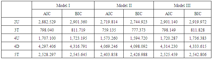
Model II of all of facilities are more accurate than Model I and Model III because the AIC values of Model II are the lowest. In addition BIC values of Model II are lower than other two model types (see Table 9, 10).Table 9. Model Fit Test for SPFs of Multi-Vehicle Collisions
 |
| |
|
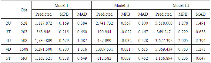
Table 10. Results of Model Validation for SPFs of Multi-Vehicle Collisions
 |
| |
|
Based on the AIC and BIC, Model II of all of the facilities should be selected. However, MPB and MAD of Model II for 2U are greater than Model I. The predicted crash frequency has more than doubled. Thus, it is not easily concluded that Model II for 2U is the best. However, other models, Model II type of 3T, 4U, 4D, and 5T are the best.
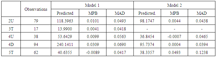
6.4. Results of the Fit Test and Validation of SPFs for Single-Vehicle Collision
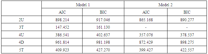
By comparing AIC of Model I and Model II, we found that Model I usually has higher value, which means that Model I is the less accurate model than Model II. Also BIC of Model 2 of 2U, 4U, 4D, and 5T are smaller than Model I. It is possible that the Model II of 2U, 4U, 4D, and 5T are more accurate to predict the single-vehicle collisions than Model I. Meanwhile, the MPB and MAD values of the Model II of 2U, 4D are closer to zero than Model I values. On the other hand, the Model I of 5T has closer values than Model II (see Table 11, 12). Table 11. Results of Model Fit Test for SPFs of Single-Vehicle Collisions
 |
| |
|
Table 12. Results of Model Validation for SPFs of Single-Vehicle Collisions
 |
| |
|
As shown Table 8, however, the regression model of 3T has the value approximately equal to zero. It means that NB regression model may not be a good estimation than a Poisson regression model. In addition, the estimation was failed to be converged in the previous step. Therefore, it is not recommended to use the estimated new SPF of single-vehicle collision for 3T in this study.
7. Conclusions
This study performed the calibration procedure of urban and suburban arterials and the development of Alabama-specific SPFs. While both calibration and development of SPFs were performed, we used the CARE data which consists of 0.01 mile roadway segments with ninety one variables including crash frequencies, AADT, speed limits and other requisite information. Even though we have detailed accident and roadway geometry, it was too difficult to apply directly on the HSM process because of lack of data and different format of data. Throughout this study, we met several obstacles that interrupted attaining our research goal. Firstly, fifty sample size was too small to obtain proper calibration factor. Thus, we constructed CI to identify sample mean properly representing the population characteristics. We derived a conclusion that fifty sample size was not large to use for this study. The next step was to find an appropriate sample size. This study referred to the calculation method from the HSM calibration study of Maryland DOT. As a result, we found the sufficient sample size required. Due to the lack of data, we could not calculate C-factor using the HSM recommendation. The required sample size are over one hundred, and 2U required at least five hundred samples. However, driveway density, on-street parking information are not included in the CARE data. Therefore, we decided to develop new Alabama-specific SPFs for urban and suburban arterials. The SPFs for multiple-vehicle collisions and single-vehicle collisions were developed. This is because the crash frequencies related to the density of driveways were not categorized in the CARE data. It was not possible to estimate the crash frequency separately. We developed three types of SPFs based on the negative binomial regression model. Total fifteen new SPFs for multi-vehicle collisions were estimated, and total ten new SPFs for single-vehicle collisions were developed in this study. Throughout model fit tests and validation step, we found 3T, 4U, 4D, 5T Model II types are the best models to predict multiple-vehicle collisions. Also, we identified that AADT has been well fitted on the predictive models than log-transformed AADT in the Alabama case. On the other hand, the estimated SPFs for single-vehicle collisions had several serious problems to use. Even though some of the new SPFs showed well suited results through the tests, there were still ambiguous results. Firstly, multiple-vehicle collision model for 2U showed an inconsistent result. Secondly, almost all of dispersion parameters are too small, even one of the dispersion parameters is approximately equal to zero. Also, 3T of Model II type was not converged during the likelihood estimation. All things considered including all of the procedures of this study, it is possible that low mean affects parameter estimation and the fit tests. Specifically, 2U has very low crash frequencies including multiple- and single-vehicle collision than other facilities. In addition, single-vehicle crash frequencies of all facilities are significantly lower than multiple-vehicle collisions. Therefore, it is necessary to identify the impact of the low mean and how to overcome the problem in the future research.
References
| [1] | AASHTO. 2010. Highway Safety Manual. Washington D.C.: AASHTO. |
| [2] | Brimley, Bradford, Mitsuru Saito, and Grand G. Schultz. 2012. "Calibration of the Highway Safety Manual Safety Performance Function and Development of New Models for Rural Two-Lane Two-Way Highways." Transportation Research Board. Wahsington D.C. |
| [3] | Brown, Henry, Carlos Sun, and Praveen Edara. 2013. "Nuts and Bolts of Statewide HSM Calibration." Transportation Research Board. Washington D.C. |
| [4] | 2014. CENTER for ADVANCED PUBLIC SAFETY. The University of Alabama. Accessed July 7, 2014. http://caps.ua.edu/care.aspx. |
| [5] | Harwood, Douglas W., Karin M. Bauer, Kare R. Richard, David K. Gilmore, Jerry L. Graham, Ingrid B. Potts, and Darren J. Torbic. 2007. "Transportation Research Board." Accessed May 15, 2014. http://onlinepubs.trb.org/onlinepubs/nchrp/nchrp_w129p1&2.pdf. |
| [6] | Hilebe, Joseph M. 2011. Negative Binomial Regression. Cambridge University Press. |
| [7] | Kweon, Young-Jun, In-Kyu Lim, Tracy L. Turpin, and Stephen W. Read. 2014. "DEVELOPMENT AND APPLICATION OF GUIDANCE TO DETERMINE THE BEST WAY TO CUSTOMIZE THE HIGHWAY SAFETY MANUAK FOR VIRGINIA." Transportation Research Board. Wahsington D.C. |
| [8] | Lord, Dominique, and Fred Mannering. 2010. "The Statistical Analysis of Crash-Frequency Data: A review and Assessment of Methodological Alternatives." Transportation Research Part A 44 (5): 291-305. |
| [9] | LP, StataCorp. 2014. STATA 13. |
| [10] | Lubliner, Howard, and Steven D. Schrock. 2012. "Calibration of the Highway Safety Manual Prediction Method for Rural Kansas Highways." Transportation Research Board. Washington D.C. |
| [11] | Mehta, Gaurav, and Yingyan Lou. 2013. "Safety Performance Function Calibration and Development for the State of Alabama: Two-Lane Two-Way Rural Roads and Four-Lane Divided Highways." Transportation Research Board. Washington D.C. |
| [12] | Michigan Department of Transportation. 2012. Accessed Febraury 1, 2015. http://mdotcf.state.mi.us/public/tands/Details_Web/mdot_hsm_mi_cal_val_spring_2012.pdf. |
| [13] | Persaud, Bhagwant, Taha Saleem, Shahzad Faisal, Craig Lyon, Yongsheng Chen, and Ali Sabbaghi. 2012. "Adoption of Highway Safety Manual Predictive Methodologies for Canadian Highways." Conference of the Transportation Association of Canada Fredericton. New Brunswick. |
| [14] | Qin, Xiao, Zhi Chen, and Kimberly Vachal. 2014. "Calibration of Highway Safety Manual Predictive Methods for Rural Local Roads." Transportation Research Board. Washington D.C. |
| [15] | Shin, Hyeonshic, Young-Jae Lee, and Seyedehsan Dadvar. 2014. "The Development of Local Calibration Factors for Implementing the Highway Safety Manual in Maryland." |
| [16] | Srinivasan, Raghavan, and Daniel Carter. 2011. Development of Safety Performance Functions for North Carolina. Raleigh: North Carolina Department of Transportation. |
| [17] | Srinivasan, Sivaramakrishnan, Phillip Haas, Nagendra Singh Dhakar, Ryan Hormel, Darren Torbic, and Douglas Harwood. 2011. "Development and Calibration of Highway Safety Manual Equations for Florida Conditions." |
| [18] | Sun, Carlos, Henry Brown, Praveen Edara, Boris Carlos, and Kyoungmin Nam. 2013. "Calibration of the Highway Safety Manual for Missouri." |
| [19] | Sun, Xiaoduan, Dan Magri, Hadi H. Shirazi, and Samrat Gillella. 2011. "Application of the Highway Safety Manual: Louisiana Experience with Rural Miltilane Highways." Transportation Research Board. Washington D.C. |
| [20] | Trieu, Vanvi, Seri Park, and John McFadden. 2013. "Sensitivity Analysis of Highway Safety Manual Calibration Factors Using Monte-Carlo Simulation." Transportation Research Board. Washington D.C. |
| [21] | Washington, Simon, Bhagwant Persaud, Craig Lyon, and Jutaek Oh. 2005. Validation of Accident Models for Intersections. U.S. Department of Transportation. |
| [22] | Williamson, Michael, and Huaguo Zhou. 2012. "Develop Calibration Factors for Crash Prediction Models for Rural Two-Lane Roadways in Illinois." 8th International Conference on Traffic and Transportation Studies. Changsha, China. |
| [23] | Xie, Fei, Kristie Gladhill, Karen K. Dixon, and Christopher M. Monsere. 2011. "Calibrating the Highway Safety Manual Predictive Models for Oregon State Highways." Transportation Research Board. Washington D.C. |
 Abstract
 Reference
 Full-Text PDF
 Full-text HTML