-
Paper Information
- Paper Submission
-
Journal Information
- About This Journal
- Editorial Board
- Current Issue
- Archive
- Author Guidelines
- Contact Us
International Journal of Traffic and Transportation Engineering
p-ISSN: 2325-0062 e-ISSN: 2325-0070
2015; 4(3): 75-83
doi:10.5923/j.ijtte.20150403.01
Improved Dynamic Route Guidance based on Holt-Winters-Taylor Method for Traffic Flow Prediction
Yousef-Awwad Daraghmi, Motaz Daadoo
College of Engineering and Technology, Palestine Technical University Kadoorie (PTUK), Tulkarem City, Palestine
Correspondence to: Yousef-Awwad Daraghmi, College of Engineering and Technology, Palestine Technical University Kadoorie (PTUK), Tulkarem City, Palestine.
| Email: |  |
Copyright © 2015 Scientific & Academic Publishing. All Rights Reserved.
Accurate short-term traffic flow prediction is necessary for the implementation of Dynamic Route Guidance as motorists need to know traffic conditions ahead. The accuracy of short-term traffic flow prediction depends on how prediction models handle traffic flow characteristics such as temporal correlation, overdispersion, and seasonal patterns. Several data mining methods have been proposed to model and forecast traffic flow for the support of congestion control strategies. However, these methods focus on some of the characteristics and ignore others. Some methods address the autocorrelation and ignore the overdispersion and vice versa. In this research, we propose a data mining method that can consider all characteristics by capturing the flow autocorrelation, trend, and seasonality and by handling the overdispersion. The proposed method adopts the Holt-Winters-Taylor (HWT) count data method. Data from Taipei city are used to evaluate the proposed method which outperforms other methods by achieving a lower root mean square error. Then the proposed method is used in a dynamic route guidance systems to enhance the efficiency of guidance.
Keywords: Autocorrelation, Holt-Winters, Negative Binomial, Overdispersion, Short-term prediction, Traffic flow
Cite this paper: Yousef-Awwad Daraghmi, Motaz Daadoo, Improved Dynamic Route Guidance based on Holt-Winters-Taylor Method for Traffic Flow Prediction, International Journal of Traffic and Transportation Engineering, Vol. 4 No. 3, 2015, pp. 75-83. doi: 10.5923/j.ijtte.20150403.01.
1. Introduction
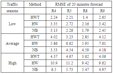
- Dynamic Route Guidance (DRG) as a part of Advance Traveller Information Systems (ATIS) aims to provide travelers with real-time information about traffic condition on routes. Due to the continuous change of traffic conditions in urban areas, travellers may select routes that will be congested during their trips. This problem can be overcomed by predicting traffic flow for a short time ahead to determine the status of all roads on routes during trips. Prediction makes DRG adaptive to the traffic changes on roads and enables travellers to choose the best routes which has the shortest travel time.Traffic flow is time series data consisting of sequences of values that are measured at equal or unequal time intervals. It has complex characteristics due to the complexity of trans-portation network particularly in urban cities which contain many intersections with traffic lights controlling traffic flow on upstream and downstream roads. These characteristics include autocorrelation as the flow time series is correlated with its values in the past and the future [1-3]. The flow may also have a trend which describes the general direction of the time series [3], [4]. Further, the flow has seasonal patterns that are repeated every week and every day [5]. Furthermore, the flow exhibits overdispersion which indicates that its variance ex-ceeds its mean [5]. Addressing these characteristics increases the accuracy of traffic flow modeling.Several data mining methods have been proposed to model traffic flow. These methods include the exponential smoothing methods such as the Holt-Winters (HW) method [4], the Autoregressive Integrated Moving Average (ARIMA) [2], [4], [6], and the Multivariate Structural Time Series (MST) [3]. Although these methods can properly model autocorrelated data with trends and the seasonality, they are sensitive to the high variation. Therefore, the accuracy of these methods may deteriorate when data become overdispersed. Furthermore, a space-time Negative Binomial regression has been proposed to model overdispersed traffic flow [5]. However, this model does not account for trends and seasonal patterns.The only forecasting method that handles time series trend and seasonality characteristics as well as overdispersion is the Holt-Winters method for count data proposed by Taylor and known as HWT count data method [7]. This method combines the double seasonal Holt-Winters with the Negative Binomial distribution. The double seasonal Holt-Winters method allows for the simultaneous capturing of small seasons that exist in large seasons such as the daily season within the weekly season. The Negative Binomial distribution allows the variance to exceed the mean during the modeling process by involving an overdispersion coefficient. The HWT count data method was shown more accurate than other smoothing methods which do not handle overdispersion [7].In this research, we propose a data mining method for modeling and forecasting traffic flow accurately. The proposed method utilizes the HWT count data method since the data used in this research are traffic flows lected from Taipei city and have all of the aforementioned characteristics. We model the weekly season as a large season and the daily season as a small season. The coefficients of overdispersion, trend, and seasonality are estimated during the training process using a likelihood function derived by Taylor [7].The contribution of this research is firstly we propose a predictive DRG system by integrating an existing ATIS with prediction. We secondly propose a method that can be used to model and forecast the autocorrelated and overdispersed traffic flows. We thirdly compare the proposed method with the HW and the space-time NB regression methods, and we show that the proposed method outperforms the other two methods because it has smaller root mean square errors. This research also defines the temporal characteristics of traffic flow as seasonal patterns and categorizes these patterns into a weekly traffic season and a daily traffic season.
2. Related Work
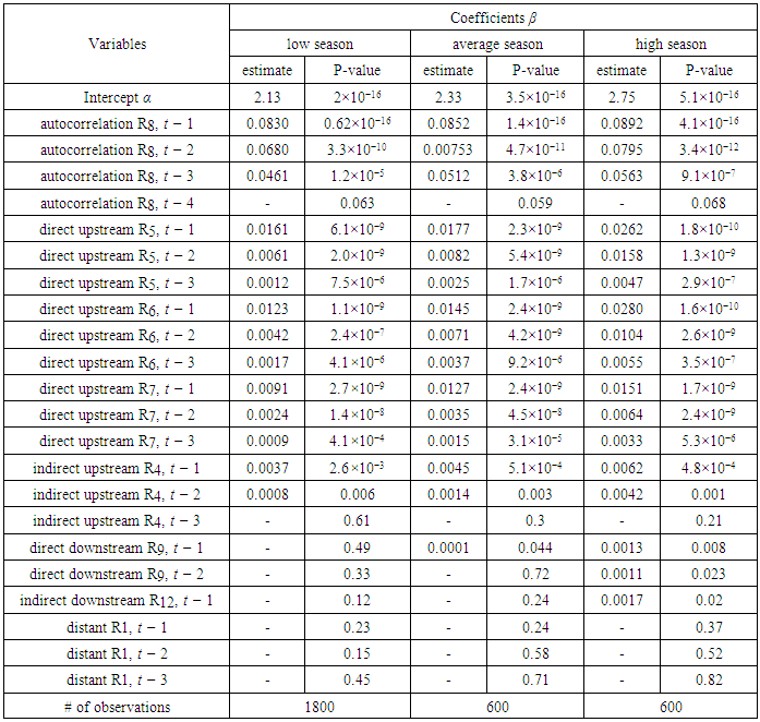
- As shown earlier, prediction is necessary for DRG. This sections reviews the most relevant methods that have been used for traffic flow forecasting in urban areas.The field of data mining consists of variety of methods that are used to model or forecast time series [8], [9]. In traffic context, the accuracy of data mining methods that are used to model and forecast traffic flow time series depends on how these methods deal with its various characteristics. Here, we give a brief review of these methods in terms of which method can properly traffic flow temporal autocorrelation, trends, seasonal patterns, and overdispersion.Several ARIMA based methods were used in the traffic context as in [2], [4], [6]. These methods were used to model different traffic variables such as speed, flow, or travel time. The strength of these methods is their ability to model autocorrelated data and capture the trends in the data. Also, these methods can be formulated as multivariate models to address the traffic conditions in several locations. However, the ARIMA based methods are usually sensitive to high variations and they become less accurate when data is overdispersed [7]. In traffic context, these methods were shown less accurate and more complex than the HW method [3], [4].The HW method was used to model autocorrelated traffic flows measured from a single site since it is a univariate method [4]. The HW can capture trends and seasonal patterns in a single time series. For more accurate results, trends and seasonal patterns from different sites were treated with a multivariate structural time series (MST) [3]. However, these methods did not address the high variation or the overdis-persion of traffic flow. Ignoring the overdispersion may cause inaccurate forecast results [10].To overcome overdispersion, a negative binomial regression that allows the variance to be greater than the mean was used to model traffic flows in Taipei city [5]. This method is called the space-time multivariate NB regression and models traffic flows from a set of correlated roads N. The multivariate space-time NB regression model can be written compactly as
 | (1) |
 is the traffic flow value of the dependent road at time t, 1 ≤ d ≤ N, α is the intercept, βi,j is the regression coefficient corresponding to road i at time j, n is the size of data, and η is the regression error vector where the error is independent of all covariates and distributed with mean = 1 and a variance= 1/φ. The results of this method were more accurate than the HW method and the MST method.The main shortcoming of the space-time multivariate NB regression method is its ability to model limited autocorrelated data and consequently being incapable of addressing trends or seasonal patterns in the data. A better option is a method that can capture trends, seasonality, and overdispersion. To achieve this, we adopted the HWT count data method derived by Taylor [7] by combining the HW with the Negative Bino-mial distribution which is popular for modeling overdispersed counts.
3. The Proposed DRG System
- We adopt an existing ATIS from Taipei city and add a prediction server so that the ATIS can provide predictive DRG services. The Traffic Control Center of Taipei city provides ATIS services as well as Intelligent Transportation Systems (ITS) services. The current ATIS consists of three blocks that are collecting data, processing data into information related to ITS and ATIS, and providing information to travellers [11]. The Taipei-ATIS relies on historical data and real time data of traffic flow and speed, which are stored in databases, to provide a web-based route planning service and information regarding traffic conditions. Traffic conditions of each road are displayed as coloured lines on the road network map.The availability of future values of traffic flow enables the ATIS to provide better route choices and more realistic traffic condition. Such future values can be obtained by the prediction server which is added to the processing data block in the traffic control center servers. The ATIS can capture the high variations of traffic and adapt its output to the new traffic condition. Fig. 1 shows the overview architecture of the proposed ATIS.
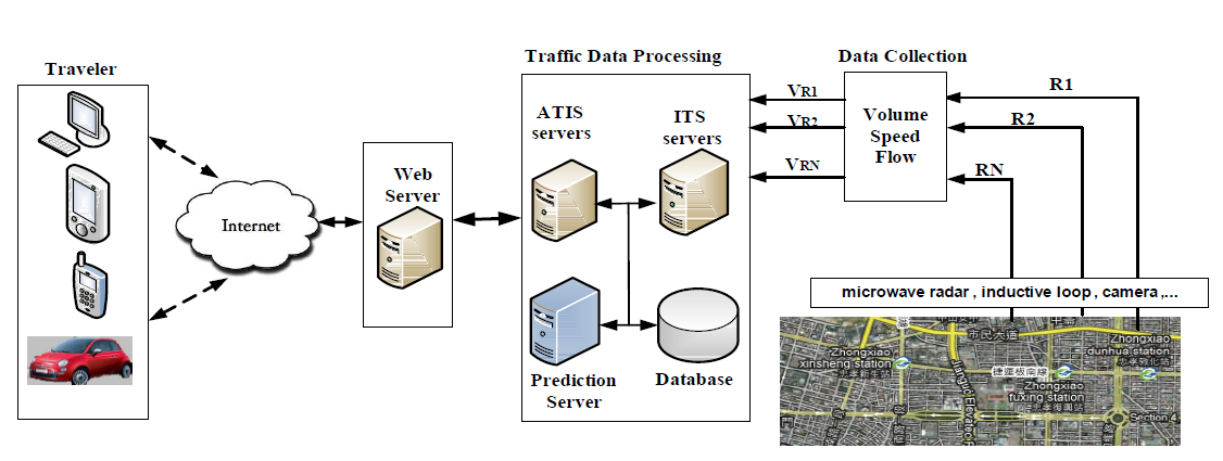 | Figure 1. The overview architecture of the ATIS that includes the proposed prediction model within the prediction server |
 | (2) |
 | (3) |
 , is assumed to be independent and identically distributed following a Gaussian distribution with mean = 0 and variance= σ2, i.e.,
  ∼ NID (0, σ2) [13]. The smoothing coefficients α, β and γ are usually restricted between zero and one, and they should be selected carefully to minimize residual errors. The equation to forecast future values,
  , is given by
 | (4) |
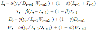 | (5) |
 | (6) |
 | (7) |
 such that
  .The resulting method is referred to as HWT count data method, and it improves the accuracy of the HW method [7]. The HWT count data method also outperforms other smoothing methods which do not account for overdispersion [7].
4. Methodology
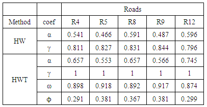
- In this section, we show how we apply the HWT count data method to the data used in this research. We also present and discuss the results of the forecasting.A. Data1) Data set: The data consists of traffic flows of 13 sig- nalized arterial road segments in Taipei city. Fig. 2 shows the traffic flow direction and the road segments. Microwave Radar Vehicle Detectors were used to record the data for 19 days from January 21, 2008 at 00:00 to February 8, 2008 at 11:58 including four weekend days. The collection of dense data with short distance between two measuring sites, 200m to 400m, and short time interval between two successive observations, two minutes, is necessary to capture all flow patterns and variations.Initially, the data were inspected and invalid records were found including missing flow values, negative flow values and zero flow values when speed is greater than zero. The invalid data resulted from detector malfunction or failure. The number of the invalid records of each road is less than 20 records per day which is not large and does not affect the accuracy of the modeling. To replace an invalid data record, we used an interpolation function that calculates the average of the preceding value and the following value of that record.2) data characteristics: The traffic flow of a selected road, e.g. R8, is represented by a time series that is plotted in Fig. 3 for 19 days and in Fig. ?? for a single day. Fig. 3 illustrates that the traffic flow has a weekly pattern which shows that the flow in workdays is different than the flow in weekends. Further, Fig. 3 illustrates that the traffic flow has daily seasonal patterns which includes intraday seasonal patterns, Fig. 4. The Intraday seasons are categorized into: a low-traffic season when the flow is less than the mean and often exists in the early morning from 00:00 to 6:00, a high-traffic season when the flow is greater than the mean and occupies time periods from 7:00 to 9:00 and 17:00 to 19:00, and an average traffic seas1on when the flow is around the mean. The flow in all roads follows the same patterns.
 | Figure 2. Map of selected roads in Taipei city |
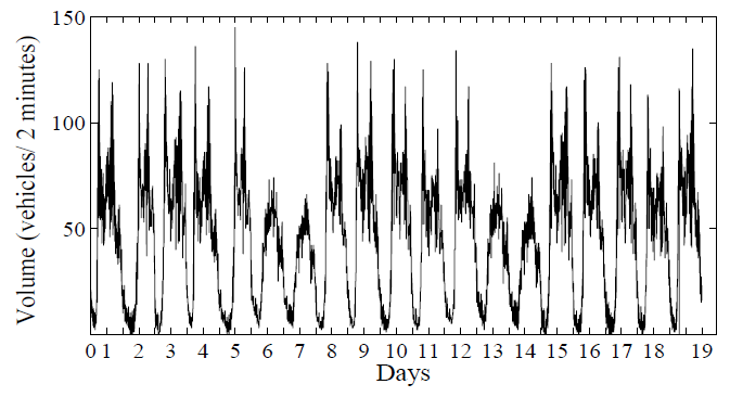 | Figure 3. The daily patterns of the traffic flow on R8 for 19 days |
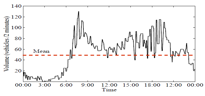 | Figure 4. The intraday seasonal patterns of the traffic flow on R8 |
|
 | (8) |
 | (9) |
 | (10) |
 | (11) |
|
 | (12) |
|
|
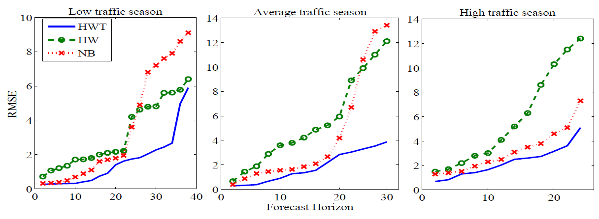 | Figure 5. RMSE against different forecast horizons during the three traffic seasons |
5. Conclusions
- The success of DRG requires accurate short-term prediction with low computational demand [17]. Accurate short-term prediction models enables DRG to provide adaptive services in real-time. Travellers will be able to select the best route pre-trip or on-trip based on current and future traffic conditions. Therefore, this paper has proposed a method for short-term traffic flow prediction in urban areas where flows are autocorrelated and overdispersed. The method addresses the most important characteristics of traffic flow including autocorrelation, trend, seasonality and overdispersion by adopting the HWT count data method. The proposed method can capture the weekly season and the daily season simultaneously. The comparison between the proposed method with the HW and the space-time NB regression methods states that the proposed method outperforms the others. This paper also has presented an ATIS that incorporates the proposed prediction model into its architecture.The limitation of the proposed method is that it only models the weekly season and the daily season. Future work will investigate the possibility of using multiple seasonal methods to model all of the intraday seasons simultaneously. Further, the proposed method needs to account for not only one road segments, but also other correlated segments. This can be achieved by deriving a multivariate HW method that can handle overdispersion and capture trends and seasonal patterns of multiple flows on different correlated roads.
 Abstract
 Reference
 Full-Text PDF
 Full-text HTML
