1. Introduction

Public railway transport plays an important role in delivering commuters to various destinations quickly and safely. Increasing the efficiency of energy consumption of this mode of travel is a significant issue facing researchers so as to enhance its competitiveness with other types of transport in the market.

In the last 20 years there has been significant development towards using energy for the traction force of electric trains efficiently. Railway transport with traditional diesel locomotives has become less attractive in terms of cost and ethical issues compared to innovative road vehicles. This is because societies have increasingly paid more attention to economic and environmental aspects of transport, such as the increasing price of energy sources, global warming and air pollution. Rapid transit trains have demonstrated their ability to compete well in terms of reliability and safety of passengers. With the increasing popularity of electrified transport the reduction of energy consumption for traction force has become a research priority.

Many researchers and practitioners have focused on these different effects with the aim of minimising the traction EC intensity of a train, either individually or in multitrain operations on a railway network and have put forward a host of viable solutions.

In this paper, transport operation will be considered in terms of the optimisation of train coasting control with developed time-driven train performance simulation and analyse of impact of different track alignments on minimising energy consumption of train for traction purposes along with improvement of train control schemes.

2. Literature Review

2.1. Optimisation of Train Coasting Control

While a train coasts, the energy consumed is much less than during traction mode. Rationally choosing the place and duration of train coasting along the railway can thus be used to decrease the traction EC for whole travel time between two stations such that braking can be avoided, hence saving the kinetic energy lost from changes in speed. In many studies of optimisation train coasting the attention has been on transport time expenditure (TTE), train traction performance and passenger comfort.

In order to achieve optimal train operation with least traction EC for the whole interstation distance a train simulation program with the principle of a coasting vector (coasting speed and coasting starting place) has been developed, which is based on train traction calculation [3]. Using this method the results show that 3% of traction EC can be saved. This can be achieved by allocating a coasting vector according to track type whenever a train reaches the coasting speed and coasting start points and this depends on passenger travel demands at different operation times on a railway line. In order to improve the results accuracy of the train coasting programme, Chang and Sim [6] suggested utilising a genetic algorithm for optimum design. They applied this algorithm in a simulation of train performance modelling in which block signals were moved in order to ensure safety in terms of the distance between two neighbourhood running trains. The elements of railway system and control actions of train were considered as genes and chromosomes, respectively.

In order to achieve optimisation of driving techniques for travelling between two stations decreasing traction EC, ensuring travel time is not exceeded and avoidance of jerky actions are the key parameters employed in the model. However, the genetic algorithm when compared with gradient algorithms is very complex for exploration when the distance between the stops is short and thus, it is suggested that coast control for mass rapid transit railways using searching methods is more appropriate [7]. Hwang [8] tried to simplify the optimisation of high-speed railway trains’ coasting control process to reduce energy consumption. Whilst research by Yang [9] involved using fuzzy clustering analyses to determine the relationships between a high-speed train’s economic speed and its traction EC as well as its travel time expenditure.

Due to the low efficiency of classical numerical optimization methods and complex train traction calculations in detailed simulation of the transport control of the train, it is difficult to ascertain accurately the optimum on-board controls for minimal traction EC. Lui and Golovitcher [10] conducted an analytical approach solved by maximal principles for relatively efficient decisions regarding the optimal control change points of a train by adopting full or partial braking and coasting or motoring with partial or full power. Based on the previous research on the effect of optimising the coasting plan of a train on its traction EC intensity, analyses of the additional impacts of traction acceleration and braking capacity of a train were made by Bocharnikov et al. [11] using simulations encompassing theories of dynamics, a genetic algorithm (GA) and fuzzy mathematics. Different coasting programs of a train for the same transport work were comparatively studied with the focus being on the changes of its travel time expenditures as well as the traction EC. The utilised GA was effectively able to avoid incorrectly adopting local optimal solutions when searching for the most energy saving coasting start points for the whole travel period. Moreover, the variables applied in the dynamic simulations were well defined by the fuzzy mathematics methods.

Figure 1. Changing of traction EC in terms of different effects

With regards to transport time schedule adherence, Kim and Chien [12] developed a train performance simulation approach to optimize the controls of a train for distinct types of track alignments so as to decrease its traction EC for a certain trip. Under some transport time constraints for a distance between neighboring stops, the most energy-saving control scheme of a train was determined according to the optimal selection of its coasting start points. More specifically, a simulated annealing approach was used to analyse the traction EC of different operations of the train for different track alignments in the transport section, which was divided into many small subsections [13]. Further, Kim and Chien [14] improved upon their work through additional consideration of the different track alignment, variable and constant speed limit, and the time constraints of an optimisation problem. The sensitivity analyses covered several different factors, including coasting position, travel time constraint, maximum operating speed, vertical depth and train weight.

2.2. Influence of Vertical Railway Track Profile

As previously clarified from the view point of the optimisation of the coasting scheme of a train, different elements of the vertical railway track profile may have varying effects on the traction EC intensity regarding the same train control action. Regarding which, effectively increasing the potential energy of down-hill along the railway line by decreasing the undulations of the track [15], effective design and utilisation of vertical railway track profile have all been found as being beneficial for decreasing the traction EC intensity. Valuable research on vertical railway track profiles has been carried out covering such factors as the driving strategy of the train driver, headway of trains, and the riding comfort of passengers (Fig.3).

Figure 2. Effects of coasting optimisation

Figure 3. Effects on vertical railway track profile in reducing the traction EC of train

Hoang et al. [16] were the first to carry out research on traction energy saving that focused on short distances between the stations along underground lines using simultaneous optimisation of vertical railway track profiles and operation of train control modes. Different slopes were related to real railway track profiles, with heuristic algorithms and dynamic programming being used to determine the slope change points of each type of gradient. Then, a simulation method was used with regard to the principles of train traction force to estimate the traction EC of a train for the whole distance travelled between station stops. It was found that the design of the energy-saving down-hill slopes on each interstation line and corresponding train operation control modes could be optimised in rational manner.

Under the assumption that urban rail transit trains are able to climb all types of gradients, Kim & Schonfeld [17] performed simulation of the different vertical track profile elements upon intensities of traction EC and the travel time of the train, whilst taking into account riding passenger comfort. According to this study, over a distance of 12000 ft (3658.5 m), a rational gradient design interstation line has significantly positive effects on the traction EC of a train. In addition, although reducing the acceleration rate increases travel time, it emerged as having a beneficial impact on traction EC intensity for the same amount of transport work.

Interested in the impacts of different radii of various types of horizontal railway track profile on the traction EC intensity of a train, Liu et al. [14] conducted a simulation using a train traction calculation. Their study showed that an increase in the traction EC intensity of a metro train can be accelerated if the curve radius is less than 300 meters. On other hand, if the radius track curve is more than 500 meters then there will be no significant on the traction EC of the train.

The speed adjustment action of the driver lags behind the change of the speed (control reminding) code of a train when the track gradient, speed limit and other constraints vary at different interstation locations. Ke et al. [1] put forward a combinatorial optimisation model to minimise the traction EC of a train. For an optimisation of the train speed trajectory for reducing a computational load on the block-layout design a max-min ant system was used. In a more recent study, Ke et al. [19] examined the optimal speed codes of a train, which can be determined for different sections of the track so as to provide an energy-saving, efficient, and comfortable transport service. In order to insure the practicability regardless of the driving techniques, the relationships between the acceleration rate and speed of the train as well as the vertical railway track profile were considered using a fuzzy process.

3. Train Performance Simulation

3.1. Traction and Braking Forces

According to Kim [1-3], a time dependent TPS model includes three parts: train traction module (TTM), track alignment module (TAM) and train control module (TCM). These modules are designed to imitate passenger train operations, such as powering, coasting, braking and cruising. They can be utilised to enhance different characteristics of train interstation movement, which can be running time, velocity and power consumed by a train, where the train control modes and track alignments might differ from location to location. These modules will continuously produce changing data about tractive efforts, resistances, the parameters of acceleration and deceleration, train speed, which all depend on the locations of a train and the profile of track alignment.

The purpose of TTM module is to generate the traction force (TF) required for a train’s movement, which takes into account current velocity, acceleration or deceleration parameters, and the placement of the train unit at any point during running time. This module computes TF which is dependent on the projected resistances for obtaining the sequential parameters of acceleration/ deceleration and planned speed. In addition, the required data of the TTM consists of static information, such as, the motor power of a train unit, number motors per train, number of passenger cars, number axles per car, total train weight and the cross-section size of a car. Whilst the variable data includes train coordinates, travel time, velocity, parameters of acceleration and deceleration, track profiles (concave, convex and level) as well as operational constraints, such as speed limit, station spacing, train time-table so forth. TF calculation is an iterative process, which involves moving a train to the projected track coordinates in discreet time of 1 second or more [1-3].

The net force to make every car movement of the train is equal to the differences between TF, denoted as F, and the sum of such factors as bearing, rolling, drag and grade resistances, denoted as R and damper constant d and spring constant (k) determine the couple forces. As shown in Equation (1) [49], represents the motion of the train during time t where locomotive of the train can be placed at either end.

(1)

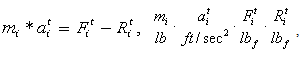
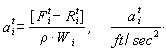
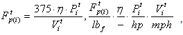
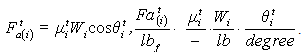
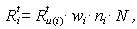
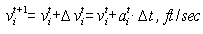
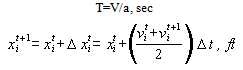
where, is car mass, is acceleration of the ith car at time t, is speed of the ith car at time t,. However, in this model it was decided to proceed without the spring and damping coefficients due to the complexity of model and the limited time for the current project.

In order to avoid slippery wheels on the track, the maximum TF at time t for the i^th car, denoted as F^t_max(i), is the minimised amount of the propulsive F^t_p(i) and adhesive F^t_а(i) forces, respectively [2, 3-5].

(2)

In Equation (2), F^t_p(i) represents the required force for the wheel to overcome the resistance and is the result of motor’s horse power P^t_i for the i^th car and motor efficiency coefficient η, which are divided by the speed of the i^th car V^t_i at time t.

(3)

where, 375 is the efficiency coefficient for converting ft-lb/sec into mi-lb/hour, which was suggested by Hay [6] and takes into account a power loss between the motor and the wheels. Usually the values of η are in the interval from 0.78 to 0.85, depending on train speed, and track conditions, which vary according to the type of gears.

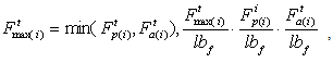
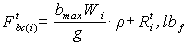
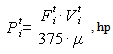
In contrast, contact between the wheel of the i^th car and rails’ surface has a friction force denoted as which is influenced by the mass of car W_i. The value of the adhesive coefficient μ_i^t depends on train speed. In the train performance simulation μ_i^t is found by the following equation [7].

(4)

The propulsion of the train can be determined by using the kinematics of whole train movement at time t inclined at an angle ϴ_i^t to the horizontal using tractive force F_i^t, resistance R_i^t and train weight W_i which is equal to zero as it is considered as center of mass. Thus, taking into account Equation (4) for the adhesive coefficient, the adhesive force F^t_a(i), which depends on the car’s weight, can be calculated from Equation (5).

(5)

Another component for determining propulsive force of train movement is resistance, which includes three important components: bearing resistance, rolling resistance and aerodynamic resistance. Bearing resistance and rolling resistance depend on the speed and weight of the train, whereas aerodynamic resistance is subject to the direction and speed of the wind as well as the size, shape and speed of the train. The modified Davis equation can be utilised to obtain the unit resistance of the i^th car at exact time t.

(6)

where, w_i is the car weight per axle, G_i^t is the gradient percentage, D_i^t is track curvature, K_i is the aerodynamic coefficient and n_i is the number of axles per car.

A parameter R_i^t represents the resistance of the i^th car at time t and can be produced from the unit resistance R^t_u(i), car weight per axle w_i, number of axles per car n_i and the number cars per train N, as follows:

(8)

The propulsive force to make a train car move is given in Equation (3.1), and is the result of the tractive force minus the resistance. It should be noted, that the propulsive force of the i^th car at time t divided by product of efficiency coefficient with train mass is acceleration a_i^t.

(9)

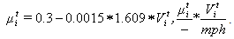
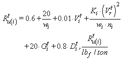
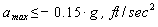
- Coefficient of rotating masses, (accepted as 1.04).

The actual braking force F^t_b(i) for the deceleration of a train can be calculated and has to be maximum value of the comfort-limited braking force F_bc or the adhesive–limited braking force F_ba.

(10)

In order to maintain passenger comfort, F_bc must not exceed a maximum value deceleration rate of b_max. Equation (8) can be rearranged for F_bc in which the maximum acceleration rate is replace by the maximum of deceleration rate.

(11)

The F_ba(i) adhesive-limited braking force refers to the adhesive factor between track rails and car wheels during the braking process of the train, which is similar to the expression in Equation (5).

For safety and passenger comfort reasons the maximum acceleration rate should not be surpassed by the actual train acceleration. In regards to the above, the suggested conditions of the maximum acceleration and deceleration rate equations (12), (13) should be used.

(12)

(13)

where, g = 32.1740 ft/sec² or g = 9.80665 m/sec² i.e. a_max= 4.8261 ft/sec² = 1.47 m/sec².

3.2. Graphing Train Speed-Time and Speed-Distance Diagrams

The train’s speed and the coordinates of locations can be calculated by knowing the acceleration and deceleration rates determined in every time interval Δt. The increment of train speed Δv^t can be easily obtained by multiplying the acceleration/deceleration rate and the time interval Δt as shown in Equation (14). The travelled distance Δx_i^t of the train is given as Equation (15).

(14)

(15)

3.3. Estimation Energy Consumption

In order to calculate power consumption P_i^t of the train to reach the speed V_i^t Equation (16) as suggested in [6] is utilised.

(16)

The planned energy consumption / regeneration rate e_i^t needed to move or during regenerative braking in time interval Δt can be found as:

(17)

It should be noted, that unit engine power is equivalent to 0.7457 kilowatts (kW) and the time interval in seconds is converted into hours. Finally, the total energy consumption E can be obtained by aggregating the energy consumption for each time interval.

(18)

where, j is the number of time intervals between two stations.

As a train regenerated energy backed to catenaries systems the total consumed energy will consists from a sum of consumed power takeaway regenerated power by regenerative braking system, however it should be assumed that all regenerated power will be fed to energy supply network.

3.4. Estimating Gradient of Track Alignment

A railway track profile consists different lengths and gradients, for which smooth connection transition parts are required, namely, sag curve and crest curve. According to Hay [6], the transition rate γ gradient should be calculated every100 ft (Equation 19) and AREA has suggested the transition rates should be estimated using coefficients of 0.05 and 0.1 for sag and crest curves, respectively.

(19)

where, G₁ and G₂ are two adjacent different gradients and L is length of the track segment.

A particular vertical track profile is converted by the track alignment module (TAM) into several track gradients which are transferred to TTM for estimating train resistance and tractive force. Then, for each user’s chosen time step the information about track grade and train position are estimated in the TTM module. The TAM module also provides maximum value of operating speed V_max to the train control module (TCM) because the train motion modes, such as acceleration, cruising, coasting and deceleration depend on the track alignment. The summarised steps of the interactions between the TAM and other modules are listed below [3].

Figure 4. Speed – time diagram of train motion with convex railway track alignment under A-V-B train control

Figure 5. Speed – distance diagram of train motion with level railway track alignment under A-V-B train control

Figure 6. Power consumption/regeneration of train along travel time in kW with convex railway track alignment under A-V-B train control

Figure 7. Energy consumption/regeneration of train along travelled distance in kW with level railway track alignment under A-V-B train control

Step 1. Identifying the number of railway track elements with different alignment and putting them between stations starting from the geometrical centre point.

(20)

where, q is the total number of track elements and j is the number of track elements in vertical alignment.

Step 2. Developing expressions for representing vertical track alignment y_j(x^t) for segment i pre-identified in step 1.

Step 3. Differentiating y_i(x^t) over distance to obtain track gradient G_j^t at track element j.

(21)

Step 4. Input G_j^t to the TTM and y_j(x^t) TCM for estimating train resistance and tractive force as well as determining train motion modes.

Step 5. Input G_j^t and V_max values to the TTM in every time interval and obtaining travelled distance (Δx^t) information from this module. It should be noted that Δx^t = x^t- x^t-1.

3.5. Train Control Schemes

The purpose of the TCM module is the determination of the appropriate train motion mode with regards to tractive force and track alignment information as calculated by the TTM and TAM. The TCM identifies appropriate different train motion modes for the various track alignments. As shown in Fig. 10., a general train control (TC) consists of motion in the acceleration regime M_a, in the first and second coasting regimes M_c1, M_c2, in the cruising regime M_V and in the braking regime M_b. It should be noted that relationship between train and time is not linear [49].

Figure 8. Convex shaped vertical railway track alignment.

Figure 9. Concave shaped vertical railway track alignment

Figure 10. Generalisation of speed profile of a train, V(t), for controlling its motion

Acceleration of a train, M_a, leaving a station and deceleration, M_b, when arriving at the station always have to be in a speed-time diagram of train motion. However, others modes of train motion are optional, varying in terms of sequence and number of times and can be integrated with the acceleration and braking regimes in a train speed diagram. For example, if the time amount for first coasting motion is excluded, the associated train control consists of acceleration, cruising, coasting and braking and so on. It should be noted that the coasting mode of train motion tends to be beneficial due to its contribution to saving energy, but it also lead to extension of travel time between stops.

The typical train control modes were summarised below according to different track alignments (Table 1).

Table 1. Typical train control modes for different track alignments

A general train control includes five motion modes and interstation travel time T can be expressed as follows:

(22)

4. Optimisation Model for Minimisation Energy

This case is designed to optimise the train control mode over single vertical track alignment (SVTA) model constrained with constant maximum operating (MOS). In order to construct this model, several important assumptions in relation to the geometry profile of the track, train control and train characteristics are made [3].

To formulate the research problem, a list of assumptions is made as follows:

1. Generalized vertical rail alignment, which may be symmetric and parabolic, connecting stations 1 and 2, as shown in Fig.11, and can be classified into three types (level, convex, and concave) of track alignments. It is worth noting that the "level" alignment indicates a tangent curve with zero gradient. Note that the terms "convex" and "concave" alignments used in this study consist of "crest" and "sag" curves, respectively, with both ascending and descending track parts. To obtain a continuous vertical track profile and associated track gradient, a general track alignment which is a function of station spacing (S), inflection points (Ip), and vertical depth/ height (δ) at halfway between two stations is assumed as:

(23)

(24)

(25)

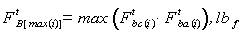
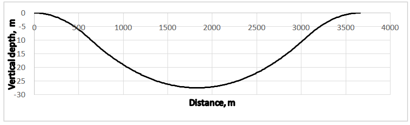
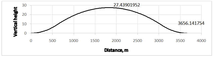
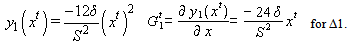
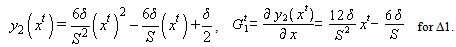
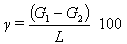
where, and represents elevations with respect to xt in metres on different segments, while is the gradient at xt in percent, and Δ₁, Δ₂, Δ₃ are 1/6, 2/3 and 1/6 of S, respectively (Fig. 11).

Figure 11. Interstation single vertical track alignment (level, convex and concave) with constant speed limit

2. The train will use the maximum TE from starting position at station 1 until it reaches the maximum operating speed (V_Max) and the maximum deceleration rate will be used when the remaining distance (RD) is equal to or less than the stopping distance (SD).

3. Four motion regimes are considered: accelerating, cruising, coasting, and braking. Note that cruising is applied where appropriate.

4. The train movement and its related forces are treated as a string mass on a route. Accordingly, the forces related to train movement, such as TF and resistance, are computed individually for the whole train as a unit.

Based on the discussion in the previous sections, the train control optimisation problem for minimising consumed energy taking in account the effects of train power, single vertical track alignment, speed limit, and maximum allowable travel time constraints, is formulated as follows:

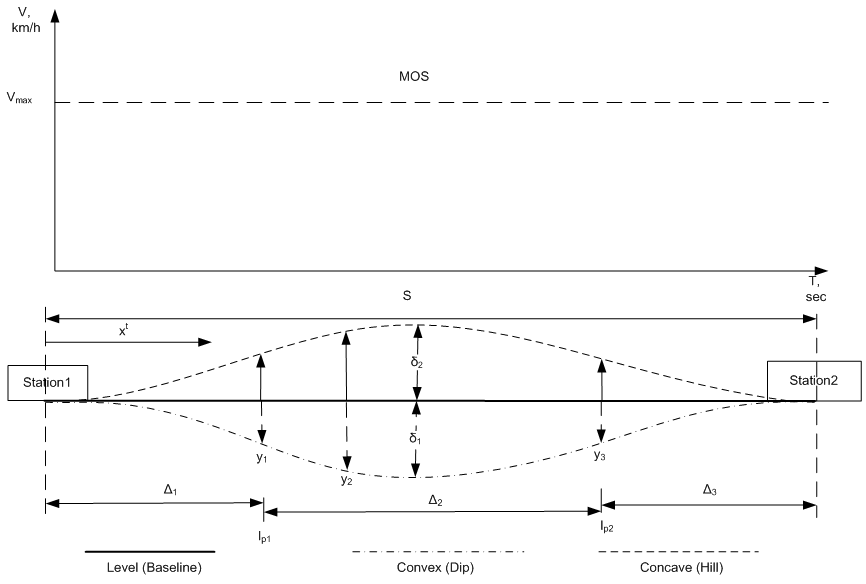
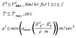
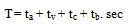
Subject to

5. Results

The aforementioned model can be used to determine the impact on energy consumption level for three types of railway track profiles (level, convex, concave) with constant maximum operating speed.

Primary static information includes 10 passenger cars of the train whose maximum motor power is 10x800 hp (8000 kW for whole train) and there is constant maximum operating speed of 107 km/hr. The maximum acceleration rate is defined by the tractive effort, which will not exceed 0.15g (i.e. 1.47 m/sec²) for passenger comfort reasons and the maximum deceleration rate must not be more than -0.15g (i.e. -1.47 m/sec²). Initial input data includes train attributes, vertical railway track profile information, operational constraints for level, convex and concave track alignment, respectively (Table 2).

Table 2. Primary static parameters for a level vertical track profile with constant maximum operating speed

In order to evaluate the optimal train control that minimises energy consumption (Table 3), the train speed-time and speed-distance diagrams in the level, convex and concave track alignments with total power consumption are estimated under the shortest travel time and optimal coasting train control modes and then compared.

Table 3. Train motion simulated results for a level railway track profile

6. Discussion

The different results of the simulation of train performance model were produced for typical track alignment (level, convex, and concave) under the shortest travel time (A-V-B) and optimal coasting train control modes (A-V-C-B) with constant maximum operation speed constraint Vmax (Table 4). An interstation distance of 3,658 metres with a constant speed of 107 km/hr MOS (Vmax) were used for all types of track alignment. The results of the simulations are summarised in the table and it is found that the level of energy consumption is significantly affected by the track alignment type.

Table 4. Results under different train control for SVTA with constant MOS

The minimum energy consumption is under the optimal A-V-C-B train control mode (90.315 kWh) on a level track alignment, which is less than the shortest travel time mode (A-V-B) on the same track alignment by 23.725 kWh (20.8%) (Fig. 12). In addition, the train motion on the level track alignment under optimal coasting train control has the second highest potential energy regeneration (11.135 kWh), which is less than the braking energy regeneration under the shortest travel time control mode by 14,305 kWh (56.23%) (Fig. 13).

Figure 12. Relationships of consumed energy, track alignment and train control modes

Figure 13. Relationships of regenerated energy, track alignment and train control modes

The minimum energy consumption is under the optimal A-V-C-B train control modes (92.669 kWh) on a convex track alignment, which is less than the shortest travel time mode (A-V-B) on the same track alignment by 21.591 kWh (18.9%) (Fig. 12). In addition, the train motion on the level track alignment under optimal coasting train control has the lowest potential energy regeneration (11.076 kWh) when compared with level and concave, which is less than the braking energy regeneration under the shortest travel time control mode by 14,387kWh (56.5%) (Fig. 13).

With concave track alignment the minimum energy consumption is 90.315 kWh under the A-V-C-B train control mode, which is less than the shortest travel time mode on the same track alignment by 23.725 kWh (20.8%) (Fig. 12). In addition to, the train motion on the concave track alignment under optimal coasting train control has the highest potential energy regeneration (11.372 kWh), which is less than the braking energy regeneration under the shortest travel time control mode by 14,056 (55.28%) (Fig. 13).

Comparing the results of simulations under the optimal coasting train control on the level, convex and concave track alignment different amounts of energy consumption and regenerated energy are found. The least energy consumption (90.193 kWh) occurs when the train motion is on a level track alignment, the second lowest is with concave track alignment (90.315 kWh) and the highest (92.669 kWh) is when there is convex track alignment. That is, the energy consumption on the level alignment is less by 2.476 kWh (2.75%) and 0,122 kWh (0.14%) than for convex and concave track alignment, respectively. While, the utilisation of optimal coasting control modes minimises energy consumption, it increases travel time from the shortest travel time by 15 sec (5.24%), 17 sec (5.99%), and 15 sec (5.24%) for level, convex and concave alignment, respectively (Fig. 14). It should be noted that the numbers in the brackets represent the increasing or decreasing of the levels of consumed power and travel time.

Figure 14. Relationships of travel time, track alignment and train control modes

7. Conclusions

In conclusion, a time-driven Train Performance Simulation has been modeled in Microsoft Excel. In the model have been taken into account the bearing, rolling resistance but also aerodynamic and gradient resistances. The speed- time a train diagram has been drown as well as graph of consumed power respect to travelled time and distance. This simulation model aimed to optimise the energy consumption of trains and evaluate impact of track alignment characteristics on its level constrained by travel time, maximum operating speed, and train technical parameters. This model could be a useful application for designing modern train control systems, such as Automatic Train Operation (ATO), to ensure efficient energy management. The results have shown that on a concave track alignment a considerable amount of energy for traction purposes can be saved, but it would require a significant amount of investment to design and produce this particular track alignment.

ACKNOWLEDGEMENTS

We acknowledge with gratitude Dr. Daniel Nankoo, my MSc project supervisor at City University London, who was always sincere and helpful for understanding the topic and guiding me through whole project. Apart from me this paper will be immerse importance for researchers who occupying with this topic. Also, I would like to thank my family member who were patient and supported me along research journey.