1. Introduction

Traffic signals have long been known to account for a significant source of delay affecting travel times in urbanized areas (Mitchell, 1968). Efforts at reducing delays at signalized intersections significantly improve total travel time experience. The ability of a traffic signal to serve a given volume of traffic through an intersection is termed its capacity. In other words, the capacity of a movement at traffic signals depends on the maximum sustainable rate at which vehicles can depart, i.e. the saturation flow and the proportion of the cycle time which is effectively green for that movement ( Akçelik, 1981). Traffic signal capacity and timing analysis techniques therefore, rely on saturation flow rates in the estimation of geometric and operational performance of signalized intersections.

Several transportation researchers have underscored the importance of saturation flow rate in signal timing design and its dependence on intersection geometry, traffic conditions, signal timing controls, and driving patterns (Akcelik, 1981; Chen, Qi, & Sun, 2014; Li & Prevedouros, 2002; Rouphail & Nevers, 2001). As such, local transportation officers are encouraged to conduct field checks on default base saturation flow rates in their localities for intersection traffic analyses.

The Highway Capacity Manual (HCM) sets out procedures for estimating actual flow rates. The actual flow rate is a scalar product of a given base flow rate of 1900 pcphpl (passenger car per hour per lane) (HCM, 2010) and an applied eleven classes of adjustment factors relating to prevailing site conditions. All, but the base flow rate relates to the given site-specific conditions. The HCM base flow value, on the other hand, represents a particular flow regime; the study intersection is located in a non-central-business- district (non-CBD) area (Le, Lu, Mierzejewski, & Zhou, 1997).This presents potential errors in the computation, when the base flow rate relating to a site is not used. In addition, the data required for the computation of the site adjustment factors are usually not readily available at the planning stage. This has often, resulted in wrong estimation of the saturation flow rates which either undermines the capacity or overestimates the actual saturation flows at intersection (Shao, Rong, & Liu, 2011; Jin et al., 2009). A study done in Japan to investigate the stochastic saturation flow rate based on the Highway Capacity Manual 2000 guidelines also showed that HCM tend to overestimate the performed saturation flow rate (Peng C. et al, 2011). This emphasizes the need for localized estimation of saturation headway and flow rate in order to optimize traffic throughput at signalized intersection.

Saturation headways are typically estimated from field measurements of the elapsed time between the 4th and 10th to 12th vehicles in a queue (Li & Prevedouros, 2002). Over the last decade, there has been a paradigm shift from overreliance on the blanket base flow rates default values provided by HCM to a more localized field based measured values due to different driver response behavior and traffic conditions at different geographic locations (Bonneson, Nevers, Zegeer, Nguyen, & Fong, 2005; Dunlap, 2005).

Several researchers conducted field studies which provided supporting evidence, that the default saturation flow rate values presented in the HCM and the measured field values obtained from these studies were significantly different (Akçelik & Besley, 2002; McMahon, Krane, & Federico, 1997). The HCM values rather tend to be conservatively high, resulting in false sense of capacity adequacy than as observed in reality. Thus, the traffic engineer should properly identify saturation flow rate that reflects the behavior of their local driving populations and update it from time to time (Joseph & Chang, 2005).

Past and recent studies in the United States indicate that saturation headways have been shortening in general, and consequently saturation flow rates have been increasing; from 2.4s observed in Los Angeles, Santa Monica, California in 1967 to 1.9s in Champaign, Illinois in 2000 (King, et al., 1976; Zegeer, 1986; Gerlough et al., 1967; R Akçelik, Roper, & Besley, 1999). This trend continuous to be observed and the variations in these headways suggest that local data be used in determining saturation flow rates. Hence, it is important for local transportation professionals to develop calibrated saturation headway models that relate to traffic behavior in their geographic regions.

HCM focuses on mean departure headway only (HCM 2010). Departure headway at each lane positions are revealed to approximately follow certain log-normal distribution (Xuexiang Jin et al, 2009). The HCM recommended headway of 1.9sec may not be the mean value at all intersections. Because of variation in driving behavior and vehicle characteristics, departure headways are usually not constant. Inaccurate estimation of departure flow often leads to inappropriate signal timing plan. Great efforts have been devoted in finding better models for effective departure flow rate (King and Wilkinson, 1977; Ruehr, 1989; Yin 2008; Yao et al ., 2009; Xuan et al., 2011). Jiyuan T. et al., 2013, built a distribution model for departure flow rate by considering the relationship with departure headway distribution and showed that the distribution models could provide richer information than the conventional mean value models and thus better serve the need of traffic simulation and signal timing planning.

R Akçelik et al., (1999), proposed an exponential model for estimating saturation flow rates, start loss and end gain times without resorting to HCM analytic procedure needed to derive saturation flows.

This research, first and foremost, established significant differences in saturation headway estimates in different geographical locations, using data from Birmingham, Huntsville, and Montgomery cities of Alabama. This was necessary to allay the assumption of homogeneity of the application of HCM base flow rate. It proceeded to develop an empirical-based exponential model equation involving few, but readily available input parameters, for estimating actual saturation headway at intersections specific to the Alabama region. This is to ensure a more consistent and reliable evaluation of saturation flow rates for planning level applications (signal timing design, capacity analysis, intersection delay and level of service analyses).

2. Data Collection

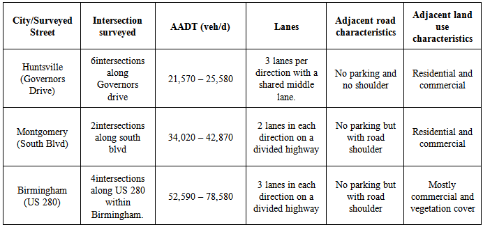
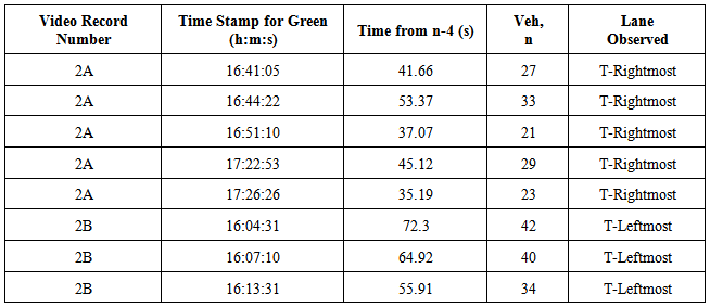
This section describes the methodology that was used in data collection and presentation. The data consisted of video records from selected intersections in three cities in Alabama State comprising Huntsville, Birmingham and Montgomery. These cities were selected such that they represented a wide range of demographic characteristics (driver aggressiveness, vehicular type population density and land use pattern) that are typical to Alabama.

Traffic data was collected via video at twenty five intersections in Birmingham, sixteen in Huntsville and thirty in Montgomery. Video traffic data was collected for 8-hourperiod per day (7:00–11:00a.m. and 3:00–7:00 p.m.) on three weekdays, viz, Monday, Wednesday and Friday. Data was collected at these times to capture peak weekday traffic. Each video record was expected to capture all turning movements; left turning movement, through movement and right turning movement.

The selection of these intersections was based on number of factors: (1) area population to examine the influence of area-type on saturation flow; (2) intersection approach annual average daily traffics (AADTs) to ensure that sufficient queues would be observed in each study cycle ( a minimum of eight vehicles were expected per cycle, HCM, 2010); (3) approach lane configuration consisting of number of through lanes with shared right turn lane, number of exclusive right turn and left turn lanes, and (4) intersection geometric characteristics to ensure that excessively skewed approaches were not included. It was to ensure that pedestrian activity did not adversely impact the flow of vehicles. A summary of the study site characteristics is shown in Table 1 and graphically presented in Figure 1. Figure 2 shows a photo exhibit of one of the study intersections. It is evident that the signal heads were not visible in the videos. Therefore, a new protocol was developed for making observations. The time and the number of vehicles crossing the stop bar were recorded when the first vehicle in the queue started rolling. For consistency purposes, the time was recorded as the front axle of each vehicle crossed the stop bar. Measurements were taken cycle by cycle. To reduce the data for each cycle, the time recorded for the fourth vehicle was subtracted from the time recorded for the last vehicle in the queue. This was then recorded as the total headway for (n-4) vehicles, where n is the number of the last vehicle surveyed (this may not be the last vehicle in the queue). The total headway was further divided by (n-4) vehicles to obtain the average headway per vehicle under saturation flow. The observations were only made for the cycles with no heavy vehicles such as tractor-trailer or dump trucks. A special data record sheet was developed to ensure uniformity and completeness in the data. A sample worksheet filled with data is shown in Table 2.

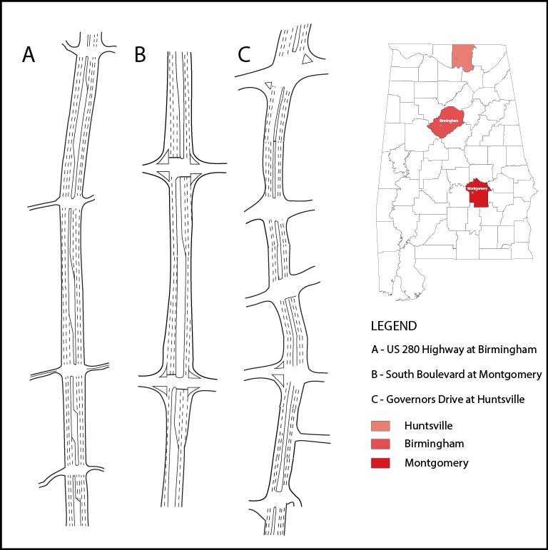Figure 1. Site location map and intersection characteristics

Figure 2. Sample screen capture from a the field video data

Table 1. Area Characteristics

Table 2. Sample Data Record Worksheet

Upon careful review of the video records, due to insufficient queue length formed at some intersections and spill backs in others, the study intersections used in the analysis were reduced to two in in Birmingham, three in Huntsville and two in Montgomery for use in determining field-observed saturation headways. A summary of the data reduced from the database including computed mean saturation headways and flow rate is presented in Table 3.

Table 3. Summary of Data Reduction

3. Methodology

This study used simple linear regression for analyzing the relationship between saturation headway and intersection related geometric and traffic characteristics. In order to identify if there exists any linear relationship between the variables, a correlation matrix was computed. The matrix is shown in Table 4. All the variables showed significant correlation at 90% significance level or higher. This justified the use linear regression for the analysis.

Table 4. Correlation Matrix of Variables Sat. Head. Through Lane Time from (4-n)s Through Lane 0.158 Time from (4-n)s -0.314 -0.231 Vehicle passed in green time -0.554 -0.198 0.957

In this study, the saturation headway was the response variable and the variables such as number of left turn, right turn and through lanes, total green time for cycle, number of vehicles crossing in the green time and the lane observed was considered the predictor variables . It should be noted that represents a matrix of predictor variables. A linear line with equation fitted the distribution using the least squares regression. The least square regression estimated a best fitting line minimizing the sum of square error i.e. the difference between the estimated saturation headway and observed.

4. Results

4.1. Comparison of Measured Headway to HCM Base

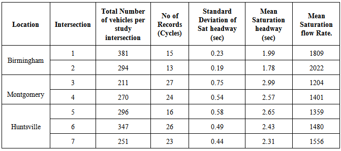
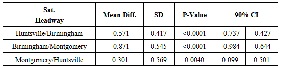
The first task was to identify, if there is any statistically significant difference between the observed saturation headway and 1.9s as recommended by HCM. This comparison was done in two different ways. Initially, one sample t-test was conducted to verify differences in the saturation headways obtained from intersections in different cities and compare it to HCM recommended headway. This analysis helps to identify unobserved heterogeneities that may exist locally affecting the saturation headway. The results of the one sample t-test indicate that for Huntsville and Montgomery the saturation headways are statistically significantly different from 1.9s recommended by HCM. The results of the test can be seen in Table 5. For Birmingham, there was not enough evidence against the hypothesis of no difference between the base headway and observed headway.

Table 5. One Sample t-test 90% Significance level SatHeadway Mean SD P-Value 90% CI Huntsville 2.477 0.604 <0.0001 2.382 2.567 Birmingham 1.915 0.231 0.7250 1.816 2.822 Montgomery 2.786 0.672 <0.0001 2.589 2.822

After identifying significant difference between the computed saturation headways and the base HCM headways, the next task was to compare if there exists any differences between the headways of different cities. As the samples collected were from three different cities, the driver characteristics and behavior is expected to be different and hence the observations can be considered independent of each other. Thus, a two-sample t test is used to identify the differences in the mean as shown in Table 6.

Table 6. Two Sample t-test 90% Significance level

The null hypothesis in all the tests was to check any probable difference between the saturation headways of different cities. However, for each of these hypothesis tests, the p-value computed was very small indicating a significant difference between the headways. This is very important finding, because using the same base headway for different cities will be clearly incorrect and resulting in the reduction for the efficiency of the intersection. Thus, this study developed a regression model to estimate the saturation headway for these cities.

4.2. Regression Model for Estimating Saturation Headway

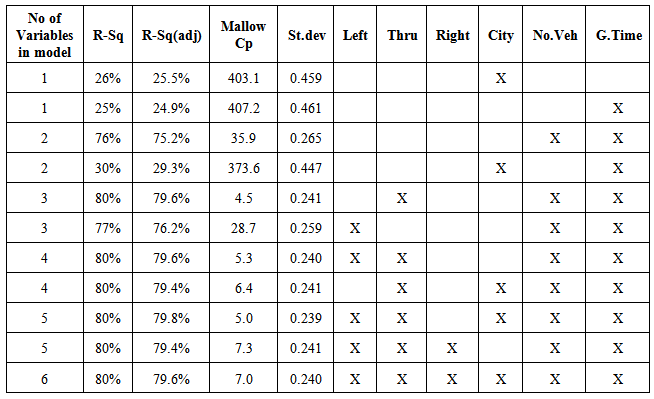
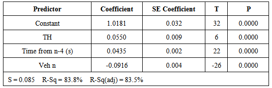
After identifying that there exists a statistical difference between the observed saturation headway and the HCM recommended headway, a regression model is developed to compute the headways given certain geometric and traffic characteristics of the intersection. Several variables were identified for study; however, not every identified variable was available. Hence some of the variables that were considered in the analysis include number of turning lanes and through lanes, city (considered as a proxy for the driver characteristics), total number of vehicles crossing the intersection and the average green time per cycle.

In order to identify which variables should be included in the model a best subset regression analysis was conducted. The best subset regression analysis uses all the combinations of the available predictor variables to identify the best combination of variables, which explains the most variability. The result of the best subset regression is given in Table 7.

Table 7. Model Variables

It is observed from the table that there are five variables which best explains the relationship between the saturation headway and the geometric characteristics of intersections.

The variables include number of left turn and through lane, total vehicle clearing the intersection, city and effective green time. A linear regression model is than developed using all the above variables. The test statistic is shown in Table 8. The final model is presented in Equation 1.

(1)

where,

H = average discharge headway

T = number of through lanes

G = effective green time

S = volume of vehicles per approach

Table 8. Sample Data Record Worksheet

The final regression model consists of number of through lanes, total green time starting the passing of fourth vehicle and the total number of vehicles clearing the intersection. The R-square-adjusted value of the model is 83.5% indicating approximately 83% of the variability in the saturation headway is explained by the estimated model. The response variable was log transformed since it gave a better fit to the model. The residual plots shown in Figures 4 – 6 indicate that the log transformation works well with the data. Figure 3 shows that most of the residuals are very close to the normality line indicating that the assumption of the normally distributed errors is not violated. However, the tail of the distribution seems skewed, which is confirmed from Figure 6. The residuals seem to be positively skewed. Figure 4 shows a funnel pattern indicating a possible violation of the homoscedasticity assumption. The least square estimates are still unbiased, although, standard errors and confidence intervals might have some effect. Therefore, this study uses a lower significance level of 90% unlike other studies, which use 95%.

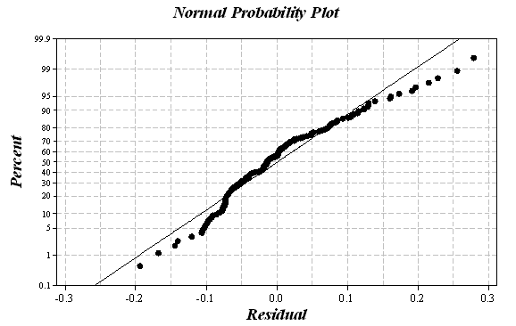Figure 3. Normal Probability Plot of Log-Normal of Saturation Headways

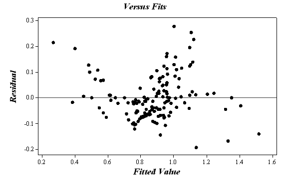Figure 4. Versus Fit Plot of Log-Normal of Saturation Headway (s)

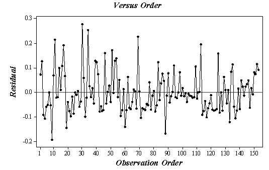Figure 5. Versus Order Plot of Log-Normal of Saturation Headway (s)

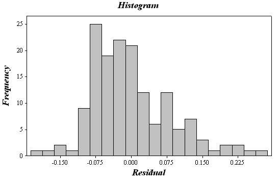Figure 6. Histogram of Log-Normal of Saturation Headway (s)

5. Conclusions

This paper analyzes the saturation headway using data from intersections in Huntsville, Birmingham and Montgomery cities of Alabama. The study compares the HCM base saturation headway with the observed saturation headways. A student t-test concludes that there exists a statistically significant difference between the saturation headways observed between the cities and HCM recommended value of 1.9s. This highlights the need for field investigation of saturation flow measurement in traffic signal planning. The exponential discharge headway equation described in this paper, therefore, presents anew possibility for more realistic estimate of discharge headway with limited input parameters for traffic modeling at planning stage. The model can be applied in scenarios where there is not enough time or resources to collect an accurate data necessary for computing saturation headways. In which case, it can give a fairly reliable value of saturation headway which can be used for planning purposes, especially at feasibility and preliminary stages of a study.

Inasmuch as the saturation headway model developed in this study can be used, however, no validation process has been done on the results. It is therefore recommended that further surveys be conducted for model validation. Again, to replicate the results outside the State of Alabama the model should be calibrated to establish discharge headway parameters in the equation.

Further research is recommended to investigate the effect adverse weather conditions and pedestrian activities on the discharge headway parameters.

ACKNOWLEDGEMENTS

The authors thank Alabama Department of Transportation for providing the initial support and funding towards conducting the traffic field surveys.