1. Introduction

Measuring traffic congestion provides the data that is used in decision-making towards congestion managementby documenting congestion information such as travel time, average speed, or delay time[1]. Travel time and delay data is perhaps the most important type of data used tocalibrate and validate the simulation model that supports Advanced Traveler Information Systems (ATIS) and Advanced Traffic Management Systems (ATMS) strategies for road capacity enhancement, such as traffic signal optimization and incident management on freeways and arterials[2-6]. Quiroga and Bullock[7] grouped the most commonly used techniques for collecting travel time data into two categories: roadside techniques and vehicle techniques. With improvement of GPS technologies, various travel time data collection procedures can be performed more efficiently. Data collection techniques for travel time and delay are usually organized in four general groups[8]:

■ The active test vehicle technique

■ The license plate matching technique

■ The passive ITS probe vehicle technique

■ New and non-traditional techniques

Since the 1920's, the test car technique has been used to collect travel time, and is still one of the most common methods. Using this technique the driver behaves like an average driver, without being below or exceeding the speed of an average vehicle in the stream of traffic. In this paper, the active test vehicle technique (also known as test vehicle technique or probe vehicle technique) is studied in three different levels of its own:

■ Manual (MAN)- recording, manually, elapsed time at predefined control points

■ The Distance Measuring Instrument (DMI)- determining travel time and distance along a corridor based upon speed

■ The Global Positioning System (GPS)- provides test vehicle position, time, and speed

The use of traditional sensors installed on major roads (e.g. inductive loops, AVI sensors)[8][9] or more recent Bluetooth sensors[10] along arterials and freeways for collecting data is necessary but not sufficient because of their limited coverage and expensive costs for setting up and maintaining the required infrastructure[11]. Moreover, traditional sensors are capable of monitoring discrete points along the most congested roadway but do not provide information about conditions on the road sections between sensors. As a relatively low-cost, high accuracy solution, GPS related data collection techniques have gained acceptance among transportation engineers and practitioners [12]. Since1997, the Delaware Department of Transportation (DelDOT), with help from the Delaware Center for Transportation (DCT) at the University of Delaware, has been using the GPS technique to collect the travel time and delay data on all major roads and highways in the State of Delaware (Figure 1). Previous studies have proven that travel time data collection using the GPS is equally accurate as the manual test vehicle method, and that it is 50% less labor-intensive[13][14]. However, there is a lack of studies to compare the three techniques. A comparative analysis of manual and GPS techniques has shown with a 95% confidence level that the difference between the manual and the GPS technique is not statistically significant[13]. Using the parametric t-test and the F-test the variances were found to be equal and the means of the methods were not significant at the two-tailed probability level.

This paper furthers this investigation and presents an extensive non-parametric statistical comparison of the data accuracies using GPS, DMI, and manual data collection techniques.

2. Experimental Data Collection Procedure

The experimental data collection method includes the design of the process and data variables. First, about a four-mile long stretch of Route 896, south of Newark, Delaware was chosen, a map of which appears in Figure 2. The main purpose of choosing this particular section was to obtain a fewconsecutive segments,each with different characteristics, to test if the segment variables (length, number of signals, curves etc.) have an impact on travel time and delay time data collection methods.

Distance on a two-lane arterial highway was divided into three segments in each direction, for a total of six segments (Table 1). Each of the three one-directional segments had slightly different characteristics: Segment 1 has a straight section with several traffic lights, Segment 2 is a stretch of road with one light in the southbound direction and with no delay in the northbound direction, and Segment 3 is a longer segment including four traffic lights and is curved at one end of the segment.

Table 1. Road segments

The data collection for each segment included measuring travel time in seconds, delay time in seconds, and distance in miles. Distance measurements obtained using the GPS and manual methods were in miles with accuracy to hundredth of a mile. Although the initial segment distance values obtained by DMI were in feet, they were converted to miles to be consistent with other measurements.

The required sample size was estimated using the recommendations of a study done by Faghri and Hamad[13]. From the given power of their sample size, it was decided to obtain thirty-two samples for each segment.

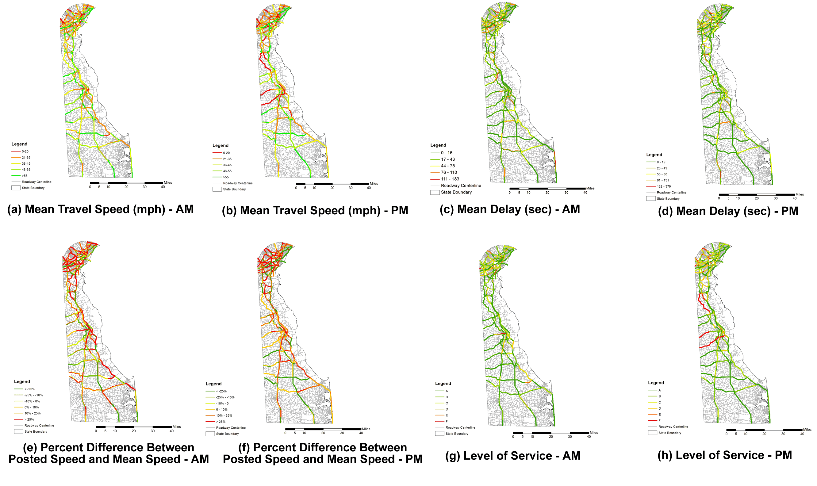Figure 1. Example of route map output from GIS

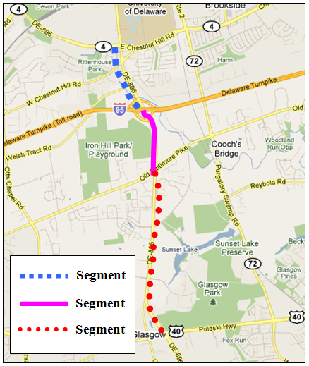Figure 2. The study area with three segments of the State Route 896, Newark, DE (Source: ©2013 Google Map)

The three data collection methods were used simultaneously, using one test vehicle with three operators randomly assigned to different methods to avoid human biases. In reality it was more complicated than that; the driver was using a stopwatch for delay measurements and reading the odometer at each control-point. One of the two remaining people was using the TDC-8 and a stopwatch for travel time measurements, and the second passenger was using the GPS unit. The data were collected during the off-peak hour from 9:30 AM to 11:00 AM during the weekdays. Each day a maximum number of four runs in each direction were completed. Upon the completion of the runs, the data were processed.

The hypothesis tested in this study is whether the three data collection methods are equal or different; therefore, a two-tailed hypothesis test will be applied, and as a result we test:

H_o: the methods are the same

H_A: the methods are different

3. Statistical Analysis of the Data

Before applying statistical tests, we must make sure that the correct statistical approach is used. Therefore, each data set has to be tested for normality to find if the underlying distribution of the samples is normal. The simplest normality tests usually indicate if the distribution is normal or not, but do not show the type of the distribution. Also a test of data independence will be performed.

The travel time, delay time, and distance data were collected simultaneously for all three methods, but we cannot evaluate normality for data obtained in series; therefore they will be evaluated in pairs: manual and DMI methods, DMI and GPS methods, and GPS and manual to compare and evaluate the behavior of the results.

3.1. Analysis for Normality

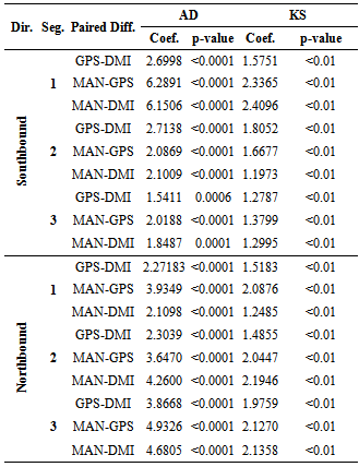
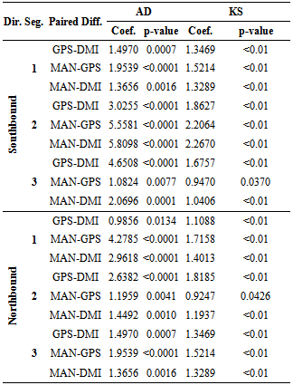
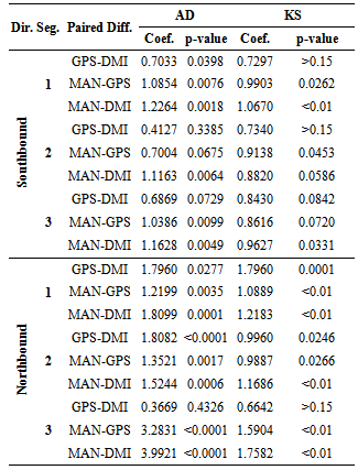
The purpose of the normality tests is to see whether there is detectable evidence that the normality assumptions for a given hypothesis test are being violated. Each test has its own set of assumptions to be held. For instance, the paired t-test assumes that the differences of the samples are independent and normally distributed. Most of the normality tests do not indicate the cause of the non-normality, but only detect that the normality assumption has been violated. It is also known that small sample sizes usually are in agreement with the normality assumption, and therefore, it isharder to detect the assumption violation.

There are several normality tests known, such as Lilliefor's, Kolmogorov-Smirnov (KS), Anderson-Darling (AD), andD'Agostino-Pearson. The most common goodness-of-fit test is the KS test, which helps determine if the sample population follows a specific distribution, and it is based on an empirical distribution function. The KS test hypothesis is defined as:

H_o: the data comes from a specific distribution

H_A: the data does not follow a specific distribution

The more appropriate normality test is the AD test. It is a modification of the KS test and has several advantages over that, including the fact that it is more sensitive on tails. The analysis in this section involves only two tests for normality: the AD and KS tests, which both are based on a cumulative distribution function[15][16].

Results of the normality tests are displayed in Table 2, Table 3, and Table 4. There we find that the majority of our data samples do not follow a normal distribution at the α = 0.05 level, either with the AD or KS test as indicated by a small p-value indicating that normal distribution is highly unlikely.

Table 2. AD and KS test for Normality for Travel Time differences

According to the p-value in Table 2, the travel time does not follow a normal distribution; therefore we reject the H_o hypothesis in favor of H_A. Also the delay time data for paired differences in the Table 3 verify that they do not meet the normality criteria. Note that Segment 2 northbound has been excluded from the analysis, as it has zero delay.

Differences of the distance measurements have weak evidence of a normal distribution too, mostly between GPS and DMI paired differences using the AD test. In this case, KS test is not used to draw conclusions about normality, using the fact that the AD test is a modification of the KS test.

Table 3. AD and KS test for Normality for Delay Time differences

Therefore, we conclude that travel time, delay time, and distance data for paired differences between GPS-DMI, MAN-GPS, and MAN-DMI are not considered normal and nonparametric statistics are more appropriate to analyze the given paired data set.

Table 4. AD and KS test for Normality for Distance differences

3.2. Analysis for Independence

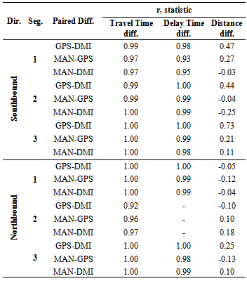
The degree to which two variables are related to each other can be measured using the Pearson Product Moment Sample Correlation Coefficient[17][18].

However, previously we have determined that our data does not follow a normal distribution; therefore, we must use the Spearman test, which is used for non-normal data. This is a test of independence based on ranks, where r_s is the correlation coefficient. The correlation value ranges between -1 to +1, where +1 indicates a perfect positive correlation between the n variables, but - 1 indicates a perfect negative relationship. There is no relationship between the variables if the correlation coefficient is zero or very close to zero. The correlation test has been applied to each data set.

From the correlation results of the travel time and delay time data in Table 5, one can clearly see that the given continuous data are closely correlated, therefore, dependent. As a result, only non-parametric or distribution-free statistics can be applied for further data analysis. Although distance measurements in Table 5 indicate little correlation between the variables, showing either weak positive or negative relationship between the data sets, non-parametric tests will also be applied to distance data.

Table 5. Spearman test for Independence

3.3. Non-parametric Statistical Tests

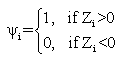
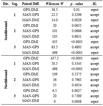
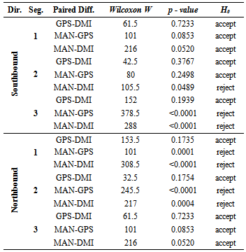
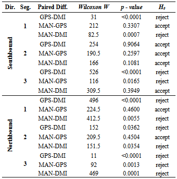
Parametric statistics assume that a given population follows a normal distribution with a mean μ, and variance σ². On the other hand, non-parametric statistics have no assumption about the underlying distribution; therefore, it is often called a distribution-free statistic[17][19]. In previous sections we determined that travel time, delay, and most of distance data are not normal and are dependent. Therefore, travel time data collection method paired data will be evaluated using the three non-parametric tests: Wilcoxon Signed Rank test, Sign test, and Minimum Chi-square test.

Wilcoxon Signed Rank Test

Wilcoxon Signed Rank test is known as the nonparametric alternative to the paired t-test. The Wilcoxon Signed Rank Test is designed to test the hypothesis about a shift in location of a median Ө in the distribution. However, there are a few assumptions to be considered:

■ the paired differences are assumed to be independent,

■ each paired difference comes from a continuous distribution that issymmetric, and

■ the paired differences have the same median.

The null hypothesis assumes that there is a zero shift of each distribution for the differences. First, the observations of the study are taken in pairs, and then the differences between each pair are calculated. The next step includes rank R_i of the differences from the smallest to the biggest, ordered by absolute value |Z₁|, ..., |Z_n| and summing the positive values to obtain T⁺ [17].

(1)

where

(2)

Table 6. Wilcoxon Signed Rank test for Travel Time Differences

We will use a two-sided test for the obtained travel time data to test H_o: θ= 0 versus H_A:θ ≠ 0. The three pairs are grouped: GPS-DMI, MAN-GPS, and MAN-DMI. The results in Table 6 show that MAN-GPS pair has the closest travel time values for Segment 1 and Segment 3. On the other hand, Segment 2 indicates a close agreement between MAN-DMI methods, showing that, in fact, the methods are equal at the 0.6831 and 0.4054 probability level. The delay time data in Table 7 shows that the GPS-DMI are the two closest related methods with probability levels of 0.7233, 0.3767, 0.1939, 0.1735, and 0.1754.

Table 7. Wilcoxon Signed Rank test for Delay Time Differences

Distance measurements in Table 8, however, show that if the distance is shorter then it is more likely the methods will perform equally, but as soon as the distance increases, the value fluctuates. We can conclude that measuring delay time using the GPS and the DMI methods is not significantly different; therefore, the manual method is the one that performs different.

Table 8. Wilcoxon Signed Rank test for Distance Differences

Table 9. Sign test for Travel Time Differences

Table 10. Sign test for Delay Time Differences

Sign Test

We will use the Signtest to see how much our travel time, delay time, and distance values fluctuate and to which side they tend to go. Here we test the H_o hypothesis that θ = θ₀ versus H_A: θ ≠ θ₀, where θ is the median of the population differences. Generally, Sign test answers how often, where the Wilcoxon Signed Rank test answers how much, our data is skewed. Sign test counts the positive differences between the paired differences. The continuous data obtained for the Sign test indicate that the closest agreement for travel time data is reached between manual and GPS techniques as indicated in Table 9.

On the other hand, delay time data indicates that manual technique has the poorest performance (Table 10), but GPS-DMI technique agrees at the 0.8036, 0.5488, 0.6636, 0.3833, and 0.4240 probability levels, which also correspond with the observations using Wilcoxon Signed Rank test. Distance measurements show a better agreement between manual and DMI techniques (Table 11).

Using the Sign test we have determined that the medians of the paired differences do not provide sufficient evidence that the differences between all the methods are zero. The data has shown that each segment and each pair of differences fluctuates for undetermined reasons. The Sign test works only on the positive and negative signs of the data, but our data represents a vast amount of zero values for travel time and delay time paired differences. As a result, in the next section we will propose an additional approach to deal with zero values.

Table 11. Sign test for Distance Differences

Dealing with Ties and Zeros (Minimum Chi-square test)

Special procedures need to be considered if the data contains ties or zero values. The ranks of the tied values need to be averaged before assigning the sign. This procedure is known as the average rank procedure[20], and it has been applied throughout the tests performed on our data.

The data in the previous sections have showed that almost every data set of the paired differences contains at least one or several zero values. Wilcoxon testcan be advised to drop the zero values before ranking the data and apply the test to the remaining values; this procedure is known as reduced sample procedure[20]. The procedure was applied to the Wilcoxon Signed Rank test and the Sign test. However, some of our data for differences between methods contain a large amount of zeros. In this case, it is suggested to apply a different procedure[17].

The procedure proposed is based on the minimum Chi-square statistic[21]. If there is no difference in the methods, the probability of a positive difference P₊(θ) is equal to the probability of a negative difference P_-(θ) = (1 – P₀(θ))/2, where P₀ (θ) = θ, for some 0≤ θ ≤1, is the probability of no difference. The Chi-square statistic for any 0≤ θ ≤1 is:

(3)

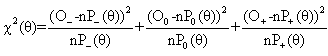
Plugging , the maximum likelihood estimator of θ, into χ²(θ), the minimum Chi-square statistic is equal to:

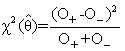(4)

For large sample sizes nthis statistic has an approximate Chi-square distribution with one degree of freedom, when the hypothesis of no difference is true. It follows that in this case,

(5)

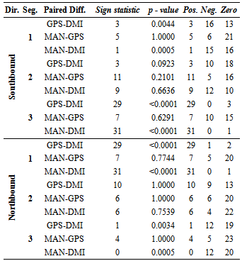
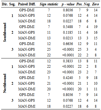
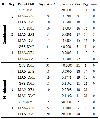
has approximately the distribution of , where Z is a standard normal random variable. To solve Equation4,first the numbers of positive and negative values for each pair between the data methods are obtained. O₊ is the number of positive signs and O_- is the number of negative signs between the paired differences.

An example of paired differences, that contains 23 zero values, is given below. We test H_o: P₊ = P_- and H_A: P₊≠ P_-.An example is given for MAN-GPS travel time of northbound Segment 3:

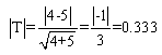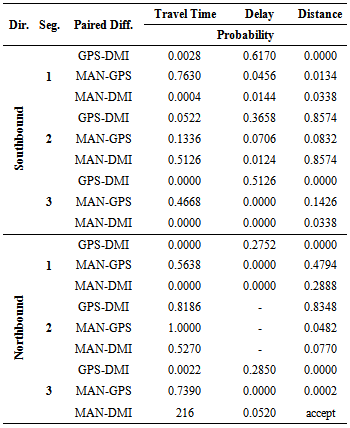
and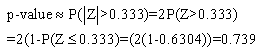

The results of the minimum Chi-square test are displayed in Table 12. According to the calculated values, manual and GPS methods for travel time measurements are not significantly different. In fact, the probability of them being equal is quite high. Comparing GPS and DMI methods and MAN-DMI methods, the results indicate that differences between the methods are not significant for Segment 2 only. For other segments, we reject the hypothesis that these data collection methods are equal. Differences between delay time measurements confirm that GPS and DMI methods are not significantly different when measuring delay times. However, comparisons between manual andGPS, as well as between manual and DMI, demonstrate that the pairs of these methods are not equal.

Table 12. Minimum Chi-Square test for Positive and Negative Differences

Distance data in the Table 12 suggests that manual and GPS method pairs, and manual and DMI method pairs, perform equally. Once again, Segment 2 has no significant difference between all methods.

3.4. Additional Segment Analysis

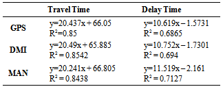
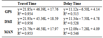
The statistical analysis has shown that for certain roadway segments of the data collection the methods follow a pattern. It has been observed that Segment 2 in both directions has less difference between the methods.

The tests possibly indicate that the methods vary according to the segment characteristics that have been described previously. The results might be a sign of correlation between the number of traffic lights on each segment and the impact on three data collection methods, as they become more apparent where segments with more traffic lights are present.

Therefore, additional linear relationships measuring travel time and delay time per mile versus number of signals per mile have been created. Table 13 represents for each method, the linear regression of travel time and delay on the number of signals per mile. Results show that R² values are fairly close to unity, which evidences the relationship between both the travel time and delay and the number of signals per mile.

Moreover, a multiple regression analysis was conducted considering average travel time and average delay time as dependent values, and the average length of each segment and the number of lights per segment as independent values. L is the average length of segment in miles, and s represents the average number of lights per segment. Results are presented in Table 14.

The result confirms that a relationship between the segment characteristics and travel time or delay time exists. However, one must be careful to draw conclusions, because the sample size of six is rather small to be sure about the results.

Table 13. Relationship between per mile Travel Time and Delay (y) and Signal Density (Number of signals per mile −x) for different methods

Table 14. Multiple Regression Analysis of Average Travel Time and Delay (y) vs. Number of Signals per Segment (s) and Average Segment Length in miles (L)

4. Conclusions and Recommendations

The Wilcoxon Signed Rank Test, with a confidence level of 95%, has accepted H_o hypothesis for following number of data pairs:

■ Travel time - 10 out of 18 data pairs

■ Delay time - 8 out of 15 data pairs, and

■ Distance - 7 out of 18 data pairs.

On the other hand, the Sign test provides following results:

■ Travel time - 10 out of 18 data pairs

■ Delay time - 7 out of 15 data pairs, and

■ Distance - 11 out of 18 data pairs.

As a result, we conclude that at least a half of the data pairs rejects the H_o hypothesis and accepts H_A hypothesis that the methods are not equal. The results show that the three travel data collection methods perform different for different data sets. We have reached a conclusion that manual and GPS methods perform equally well when collecting travel times on any of the segments. When conducting delay time studies, the GPS and DMI methods perform equally well. The manual method, assumingly, includes the difficulty of precisely reading the car's odometer, which is needed when estimating a speed of 5 mph and below.

Distance measurements, using the three methods, indicate that manual-GPS and manual-DMI methods perform equally well. However, because we have rounded distance values for DMI to match the decimal places of odometer readings, we may get insufficient results to correctly conclude which method is performing better. The initial distance measurements collected by DMI represented rather close values in feet, sometimes ranging for only a couple of feet.

On the other hand, the GPS collects the position data based on latitude and longitude, therefore a flat surface. Every great change in roadway grade introduces a small error in GPS distance measurements. Nevertheless, according to the statistical analysis, we would suggest the GPS method as the primary travel data collection method because we are interested in travel time and delay time consistent measurements.

The comparison of the travel time data methods evaluated in this research, provided information about differences between the methods. It also indicated that the differences could be related to the road segment characteristics. However the sample size was not sufficient to make the final conclusions in this regard.

An additional research could be conducted to investigate if the travel time method variations are based on road characteristics. This analysis could also be carried out comparing method performance during peak hour and compare with the off-peak hour performance. Also some odd results obtained could be attributed to rounding of the data and thus, it would be useful to perform more intensivedistance measurement comparison, and use the obtained values without data rounding.

ACKNOWLEDGEMENTS

This work was partially supported by the Delaware Center for Transportation (DCT) co-sponsored by the University of Delaware and the Delaware Department of Transportation. The authors express their sincere gratitude to DCT for providing their extensive data sources.