Oluwole O. O
Mechanical Engineering Department, University of Ibadan, Ibadan
Correspondence to: Oluwole O. O , Mechanical Engineering Department, University of Ibadan, Ibadan.
| Email: |  |
Copyright © 2012 Scientific & Academic Publishing. All Rights Reserved.
Abstract
Abtract In designing automobile suspension, response analysis is an important tool. In this paper, the response analysis of the auto suspension to various road conditions is studied using MATLABR tools and SIMULINK. The suspension system was modeled as a combination of dashpot and spring system in parallel attached to the auto body. Laplace transforms were used in obtaining transfer functions from the ordinary differential equations which described the system. The system, a second order open loop with a unity feed back ‘type 1’system was subjected to different inputs and the response was studied using Matlab inbuilt commands and SIMULINK. The system was observed to be stable to frequency input using the Nyquist diagram. Very fast settling time was observed for the responses. It was observed that it was much easier to design compensators for the system using the Matlab commands. Using MATLAB root locus plot, the system could be re-designed by choosing new locus points and the new gains and damping ratios could be obtained. With the rlocfind command, the gains in the graphics window and the damping ratio could be found as well. With this a better design of the system could be obtained by compensating the system. This brings a dynamism into the design system.
Keywords:
Response, Auto Suspension, Transfer Function, Design
1. Introduction
Automobile suspension system containing the damper and spring system serve the purpose of absorbing shocks due to road incongruities thereby making our ride pleasant. Other method of studying the system include the Finite Element Method(FEM). However, this is very cumbersome and weeks of programming and are needed to fully study system of response of system to various inputs. With the advent of control engineering software like Matlab, the process of design has been greatly simplified and stimulating. This work studies the use of Matlab and Simulink in studying auto body’s transient response to various types of road incongruities and how this is important in Engineering Education.
2. Methodology
The automobile suspension system was modeled as a combination of dashpot and spring in parallel attached to the auto body. Mathematical equations for motion of the system was formulated and the transfer functions derived using Laplace transforms. The transfer function was analysed to obtained its various parameters.The transfer function was then subjected to various probable road inputs. These are, step input, impulse, ramp and sinusoidal.
2.1. Mathematical Derivation of System Equations
Figure 1 shows a simplified schematic diagram of the auto suspension system. During motion, the vertical displacement of the tires put the auto suspension system into motion. The motion Xi at point P is the road input to the system while the vertical motion of the auto- body, XO is the output. This vertical motion of the auto-body is what the driver and the occupants feel. 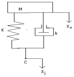 | Figure 1. Simplified auto-suspension system |
The equation for the system motion is 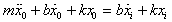 | (1) |
Taking transforms of (1) and inputting zero initial conditions gives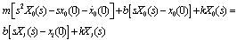 | (2) |
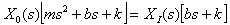
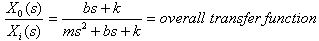 This overall transfer function describes a linear second order ‘type 1’ unity feedback system which can be represented in block diagrams as shown in Fig.2.
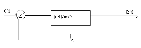 | Figure 2. Block diagram of the auto –suspension system |
The forward transfer function is (bs+k)/(ms2) while the feedback is unity. Values used for the simulation were; m= 1000Kg; b= 20KN-s/m; k=500KN/m2.
2.2. Using Matlab in Response Analysis
Various Matlab commands were used in response analyses of the auto-suspension system. Inputs were step input, impulse, ramp and sinusoidal.
2.2.1. Unit Step Response
For unit step response i.e. R(s)=1/s at t>0 ,the use of the command step(num,den) gave the desired result.
2.2.2. Unit Impulse Response
The impulse command has R(s) =1;Using impulse(num,den), the graph was plotted.
2.2.3. Unit Ramp Response
Ramp response is represented by R(s)=1/s2Since Matlab has no direct ramp command, the step command can be usedThe step command of G(s)/s is obtained where G(s) is the overall transfer function for the system. Altenatively, the command lsim(num,den,r,t) OR lsim(A,B,C,D,u,t) could be usedWhere r and u are the input time functions. The command goes thus:num=[0 20 500];den=[1 20 500];t=0:0.005:0.4;r=t;y=lsim(num,den,r,t);plot(t,r,'-',t,y,'o')Fig.5 shows the result of the unit ramp response.
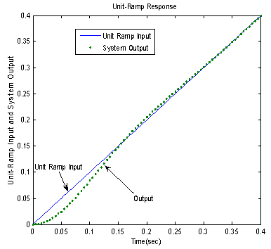
2.2.4. The response of the steady-state of the system to sinusoidal Input
The response of the system to sinusoidal input was studied using the Bode plot. The Nyquist and Nichols plots gave same results. Use was made of the command Bode(num,den) to get the Bode diagram.
2.3. Using SIMULINKR in Response Analysis
In using Simulink, it was important to obtain the poles first using the rootlocus plot. This plot gives the open loop zero and open loop poles for the system. These values are input into the transfer function property forms.
2.3.1. Root locus plot of (20s+100)/(s2+ 20s+500)
The rootlocus plot(Fig.3) was obtained by using the following commands:num=[0 20 500];den=[1 20 500];rlocus(num,den)The root locus plot showed the open loop zero and open loop poles for the system.These could be observed to tally with the complex conjugate open loop poles(roots of s2+20s+500) which were obtained by using the following procedure.b=[1 20 500];roots(b)ans =-10.0000 +20.0000i-10.0000 -20.0000i>> a=[20 500];>> roots(a)ans = -25Values obtained were:Open loop zero: s= -25Open loop poles: s=-10j20Poles (-10+20j and -10-20j ) were input into the transfer function property form. The simulink flow diagram was set up(Fig.4) and the simulation started. Results of different input signals were obtained.
3. Results and Discussion
3.1. Results
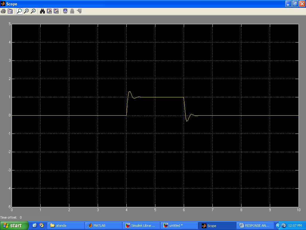
Results of the system responses to different inputs using Matlab commands are presented in Figs. 5 -11. The response to step input(Fig.5) showed a rise_time of 0.043s, peak_time = 0.11s, a maximum_overshoot of 0.3305, settling_time of 0.34s, final value of 1 and a peak amplitude of 1.34. The response to an impulse input (Fig.6)showed a peak amplitude of 20.4 at time of 0.011s and a settling time of 0.383s. The response to a unit ramp input(Fig.7) showed the a good response output. Figs. 8 and 11 showed good response to sinusoidal inputs while Figs. 9 and 10 showed very sharp initial rise time for sudden steep inputs. Fig. 12 -14 shows the frequency response plots using Bode, Nyquist and Nichols diagrams. Delay margins to frequency response was as small as 0.057s. Closed loop was stable. The values obtained showed the system stability to different sinusoidal inputs.The system responses to different inputs using SIMULINK are presented in Figs. 15-22. Fig.23 presents the use of the signal generator in building a signal. The results followed the same pattern obtained using Matlab commands.
3.2.Discussion
3.2.1. Response to various inputs
Response to the various inputs (Figs.5-11)showed a fast rise time and settling time. This showed that there is good compensator in the system. 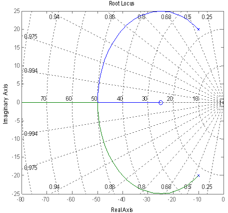 | Figure 3. Root locus plot of (20s+500)/(s2+20s+500) |
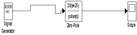 | Figure 4. Simulink flow diagram with a signal generator, the transfer function and the scope |
 | Figure 5. Response curve to a step input |

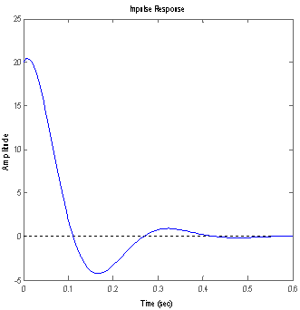 | Figure 6. Response to impulse input |
3.2.2. Response of the Steady-State to Sinusoidal Input
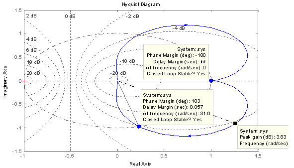
The response of the steady-state of the system to sinusoidal input was studied here. The frequency of the input signal was varied and the response to this input by the system at steady state was studied here. The Bode, Nichols and Nyquist diagrams reveal the same response to sinusoidal inputs with varying frequencies. The system studied showed stability. The Nyquist plot is a polar plot of the frequency response . We could observe the same values obtained in the Bode plot are replicated here: Peak Response: Peak gain=3.82Db at frequency of 18.9rad/secMinimum stability Margins:Phase margin=103deg. At a frequency of 31.6 rad/sec with a delay margin of 0.057sec showed that the closed loop is stable.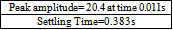
 | Figure 7. Response to a unit ramp input |
 | Figure 8. Response to a sinusoidal input sin3 t |
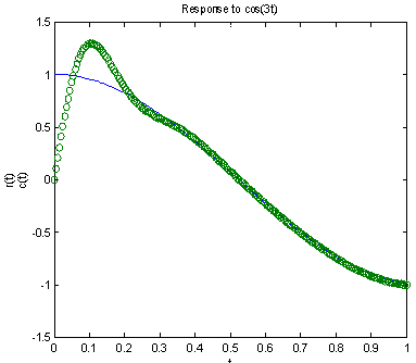 | Figure 9. Response to cos3t input |
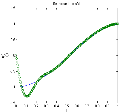 | Figure 10. Response to cos3t input |
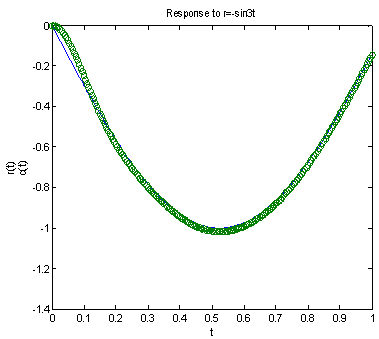 | Figure 11. Response to -sin3t input |
3.2.3. Modeling, simulating and Designing With Matlab
In the root locus plot (Fig.3), the system could be re-designed by choosing new locus points and the new gains and dampiong ratios could be obtained. With the rlocfind command, the gains in the graphics window and the damping ratio could be found as well. With this a better design of the system could be obtained by compensating the system. This brings a dynamism into the design system.
3.2.4. Modeling, simulating and Designing With Simulink
With Simulink, the user has to obtain the poles first using the rootlocus plot. This plot gives the open loop zero and open loop poles for the system. These values are then input into the transfer function property forms. Thus, it is important when using Simulink to work with both the rootlocus plot and the Simulink transfer forms. It is the input into the transfer functions that brings out the responses of the system to various input signals(Figs.15-22). Input signals can be obtained using the signal buider (Fig.23). 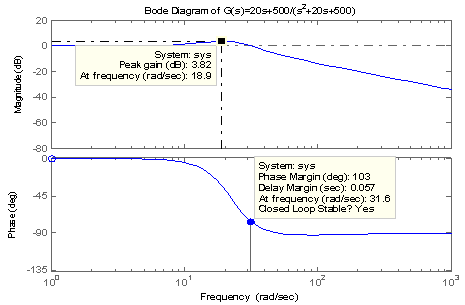 | Figure 12. Bode diagram for (20s+500)/(s2+20s+500) |
 | Figure 13. Nyquist plot for for (20s+500)/(s2+20s+500) |
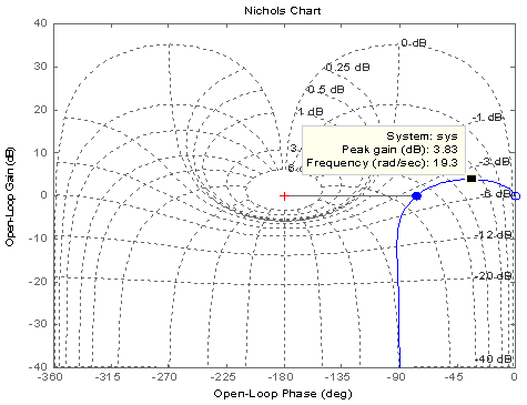 | Figure 14. Nichols plot for for (20s+500)/(s2+20s+500) |
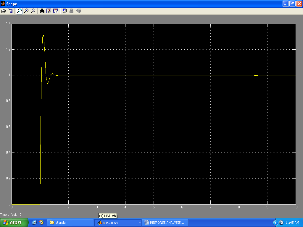 | Figure 15. Response to step input response at a step time of 1 sec |
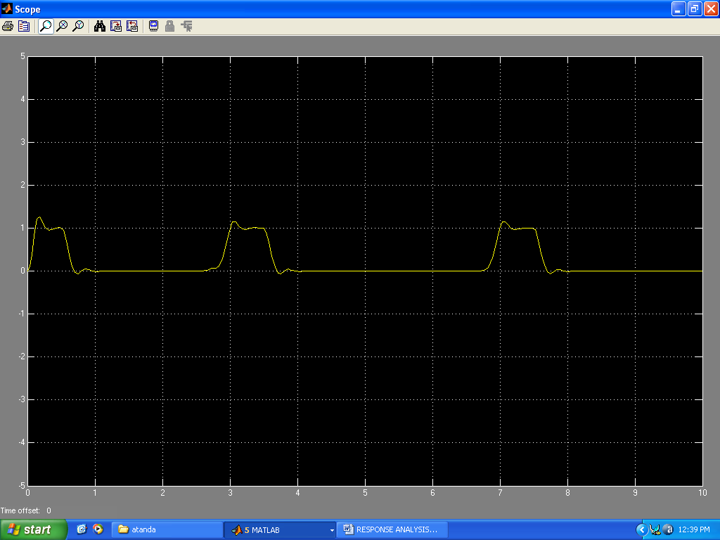
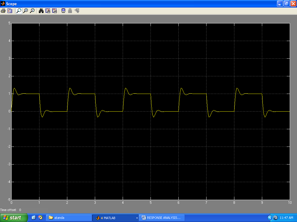 | Figure 16. Response to pulse inputs( undulating layers on road surfaces) |
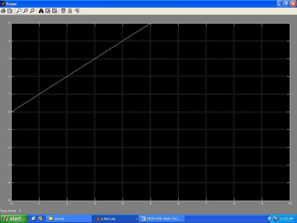 | Figure 17. Response to ramp input of slope 1 |
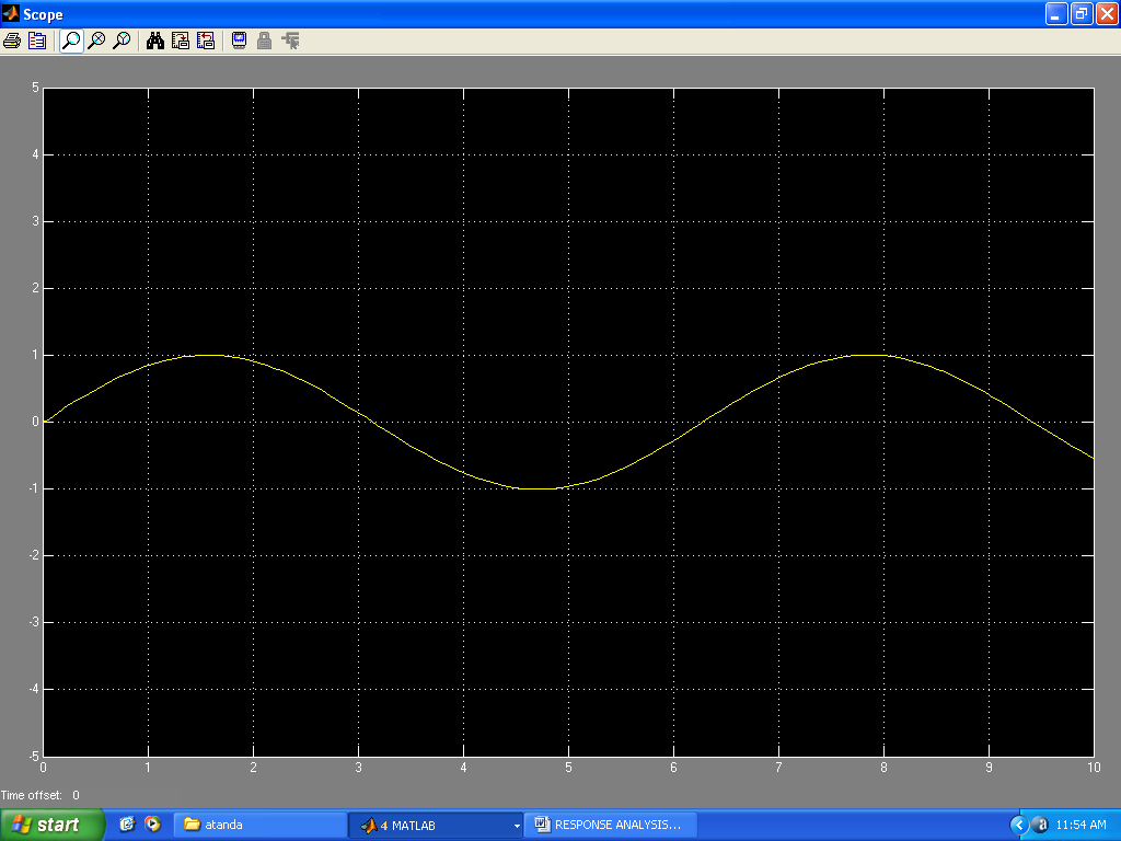 | Figure 18. Response to sinusoidal input(bumps and depths on road surfaces) |
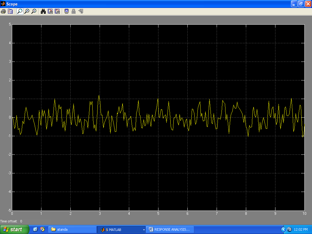 | Figure 19. Response to random inputs |
 | Figure 20. Response to square wave inputs |
 | Figure 21. Output of Sharp square input and descent |
 | Figure 22. Response to no input (smooth road) |
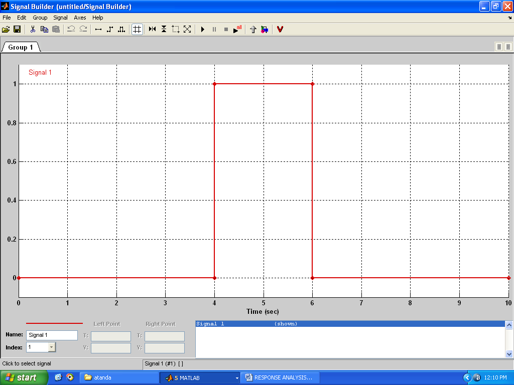 | Figure 23. Use of signal builder for input signals |
4. Conclusions
Auto-suspension system for compensators using Matlab commands and simulink has been done in this work. Using MATLAB root locus plot, the system could be re-designed by choosing new locus points and the new gains and damping ratios could be obtained. With the rlocfind command, the gains in the graphics window and the damping ratio could be found as well. With this a better design of the system could be obtained by compensating the system. This brings a dynamism into the design system.With Simulink, the user has to obtain the poles first using the rootlocus plot. This plot gives the open loop zero and open loop poles for the system. These values are then input into the transfer function property forms. Thus, it is important when using Simulink to work with both the rootlocus plot and the Simulink transfer forms. It is the input into the transfer functions that brings out the responses of the system to various input signals. Input signals can be obtained using the signal buider.
References
| [1] | Ogata.K (2002) ‘Modern Control Theory’ p.131 |
| [2] | Bandyopadhyay.M.N(2003) ‘Control Engineering’ Prentice –Hall of India.p.84 |
| [3] | WIKEPEDIA(2012) ‘unsprung mass’ en.wikepedia.org/wiki/Unsprung_mass |
| [4] | NPL(2012) ‘Optimal road hump for comfortable speed reduction’ www.npl.co.uk/ |
| [5] | ieee (2012) ‘Analysis of vehicle rotation during passage over speed control road’ ieeexplore.ieee.org/ |
| [6] | Arrb(2012) ‘Roughometer –II with GPS’ www.arrb.com.au |
| [7] | Popcenter(2012) Problem guides’ www.popcenter.org |
| [8] | Ehow(2012) ‘Bad Car struts behavior over bumps’ www.ehow.com |
| [9] | Ite(2012) ‘Comparative study of speed humps’ www.ite.org |
| [10] | SCCS (2012) Speed bumps and auto suspension analysis’ www.sccs.swarthmore.edu |
| [11] | Managemylife(2012) ‘How to make a car comfortable and quiet’ www.managemylife.com |
| [12] | Pikeresearch(2009) ‘Bumps and Toyota’s Gree auto Dominance’ www.pikeresearch.com |
| [13] | SAGEPUB(2012) ‘Effect of obstacle in the road to dynamic response of a vehicle passing over the obstacle’ www.sagepub.com |
| [14] | CARTECHAUTOPARTS(2012) ‘Car coil springs’ www.cartechautoparts.com |
| [15] | NACOMM(2012) ‘Vehicle chassis analysis’ www.nacomm03.ammindia.org/articles |
 Abstract
 Reference
 Full-Text PDF
 Full-Text HTML